You already know linear regression. Or you did, once. You learned \(y = X\beta + \varepsilon\) in a statistics class, ran it in Excel or Python, got a table of coefficients and \(p\)-values, and moved on. That knowledge is the foundation for everything in this chapter.
What we are going to do here is take that familiar model and rebuild it as a Bayesian model in PyMC. You will see that the answers barely change — the posterior means will land right on top of the OLS estimates. But the questions you can ask become richer. Instead of a single best-fit line, you get a distribution over regression lines. Instead of confidence intervals derived from asymptotic theory, you get the full posterior uncertainty over every parameter. And instead of a framework that struggles with outliers, missing data, and small samples, you get one that handles them naturally.
The payoff is not dramatic for simple problems. That is the point. Start where the answers are easy to verify, so you can trust the machinery when the problems get hard.
3.1 OLS Refresher
Linear regression models the relationship between a response variable \(y\) and one or more predictors \(X\) as:
The Ordinary Least Squares (OLS) estimator finds the \(\hat{\beta}\) that minimizes the sum of squared residuals. In matrix form, the closed-form solution is \(\hat{\beta} = (X^\top X)^{-1} X^\top y\). No iteration, no tuning — plug in the data and out comes an answer. That simplicity is what makes OLS the workhorse of applied statistics.
But notice the assumptions baked into that formula. The errors \(\varepsilon\) are normally distributed, have constant variance (homoscedasticity), and are independent of each other. When these assumptions hold, OLS is hard to beat. When they break down — outliers, heteroscedasticity, correlated errors, small samples — the guarantees evaporate. Keep that in mind as we move through the chapter.
Statsmodels gives you OLS in a few lines. Let us generate some data we can use throughout the chapter. We will simulate a simple relationship: house price (in thousands of dollars) as a function of square footage, with Gaussian noise.
                            OLS Regression Results
==============================================================================
Dep. Variable:                  price   R-squared:                       0.918
Model:                            OLS   Adj. R-squared:                  0.917
Method:                 Least Squares   F-statistic:                     876.0
Date:                Sat, 02 May 2026   Prob (F-statistic):           3.64e-44
Time:                        20:06:58   Log-Likelihood:                -379.30
No. Observations:                  80   AIC:                             762.6
Df Residuals:                      78   BIC:                             767.4
Df Model:                           1
Covariance Type:            nonrobust
==============================================================================
                 coef    std err          t      P>|t|      [0.025      0.975]
------------------------------------------------------------------------------
const         34.1527     10.589      3.225      0.002      13.072      55.233
sqft           0.1563      0.005     29.598      0.000       0.146       0.167
==============================================================================
Omnibus:                        3.950   Durbin-Watson:                   1.522
Prob(Omnibus):                  0.139   Jarque-Bera (JB):                3.155
Skew:                           0.411   Prob(JB):                        0.207
Kurtosis:                       3.520   Cond. No.                     6.76e+03
==============================================================================

Notes:
[1] Standard Errors assume that the covariance matrix of the errors is correctly specified.
[2] The condition number is large, 6.76e+03. This might indicate that there are
strong multicollinearity or other numerical problems.
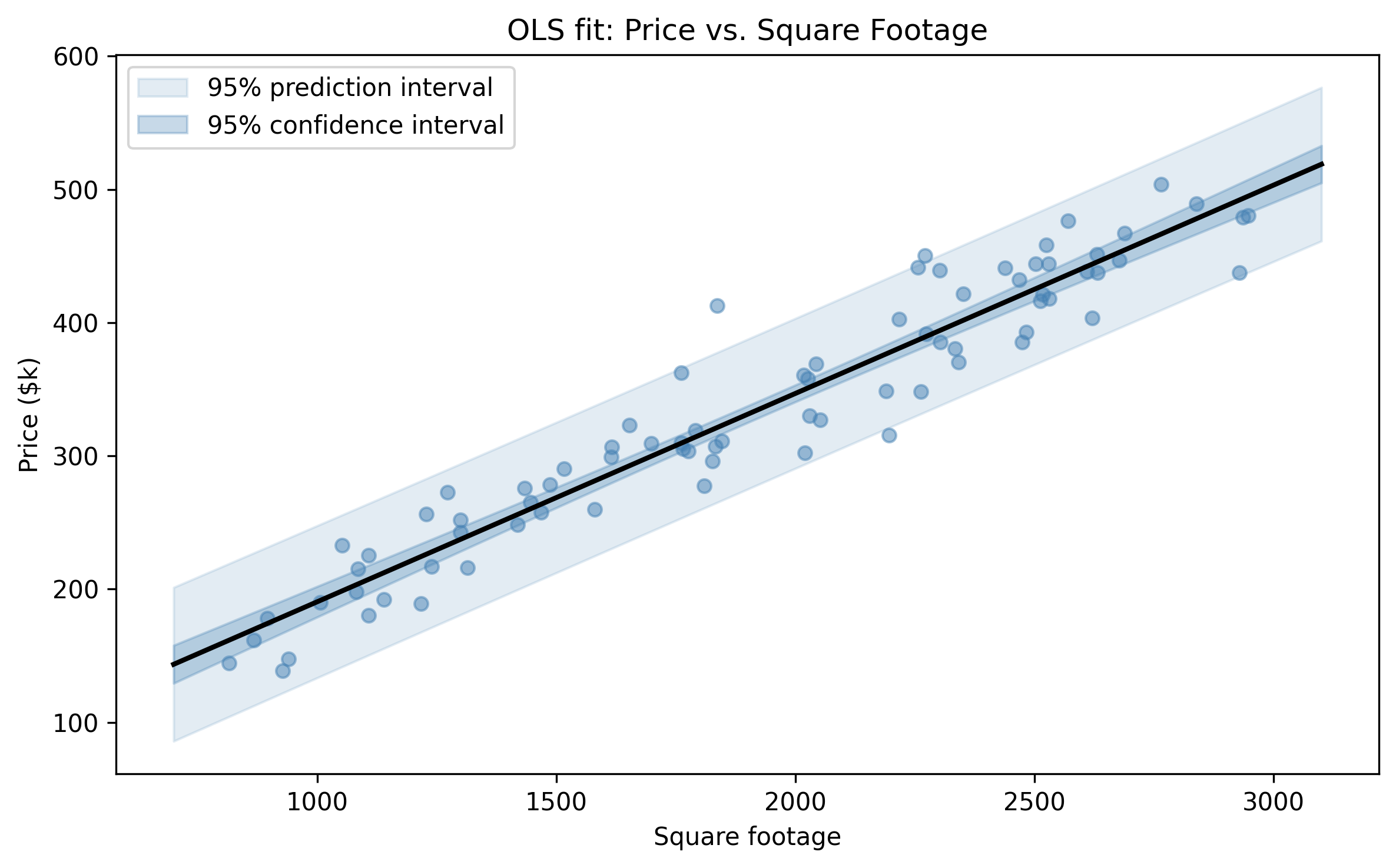
The summary gives you point estimates for the intercept and slope, their standard errors, \(t\)-statistics, \(p\)-values, and 95% confidence intervals. For this clean, well-behaved data, OLS works perfectly. The estimates should land close to the true values we used to generate the data (\(\beta_0 = 50\), \(\beta_1 = 0.15\), \(\sigma = 30\)).
Figure 3.1: OLS regression line with 95% confidence band.
This is the baseline. Everything that follows should reproduce these results — and then go beyond them.
Take a moment to notice what OLS gives you: a single best-fit line, a table of standard errors derived from the residual variance, and confidence intervals computed from the \(t\)-distribution. These are all functions of the data and the model assumptions. If the assumptions hold, they are exactly right. If they do not, you have no easy way to know how far off they are. The Bayesian approach will give us a different way to think about these same quantities.
3.2 The Bayesian Linear Model
The Bayesian version of linear regression uses the same likelihood:
The difference is that we place prior distributions on the unknown parameters \(\beta_0\), \(\beta_1\), and \(\sigma\). Instead of computing a single point estimate, Bayes’ theorem gives us a posterior distribution over all three parameters simultaneously:
Think of it this way. OLS draws one line through the data — the line that minimizes squared error. The Bayesian model draws many lines, each weighted by how well it explains the data and how plausible it is under the priors. The posterior is the full collection of plausible regression lines, not just the single best one.
For weakly informative priors — priors that rule out absurd values but do not strongly favor any particular answer — the posterior will be nearly identical to the OLS result. That is not a bug. It is a sanity check. The priors are doing their job: letting the data speak while gently constraining the model to reasonable territory.
Each prior says: “I do not know the exact value, but I can rule out values that are physically nonsensical.” The normal priors on \(\beta_0\) and \(\beta_1\) are centered at zero with wide standard deviations. The half-normal prior on \(\sigma\) forces the noise scale to be positive. These are not strong opinions — they are guardrails.
A common worry at this stage is: “Am I not biasing the results by choosing priors?” With weakly informative priors like these, the answer is barely. The prior \(\mathcal{N}(0, 200)\) on the intercept says the intercept is somewhere between roughly \(-400\) and \(400\) — hardly a controversial claim for house prices in the hundreds of thousands. The data will overwhelm these priors. If you picked a prior of \(\mathcal{N}(0, 0.01)\), that would bias the results. The distinction between “weakly informative” and “informative” priors is one of the most important practical skills in Bayesian modeling, and we will explore it directly in Exercise 1.
3.3 Building It in PyMC
Now we translate that generative model into PyMC code. Every line maps directly to a line in the math above.
import pymc as pmimport arviz as azwith pm.Model() as linear_model:# Priors beta_0 = pm.Normal("beta_0", mu=0, sigma=200) beta_1 = pm.Normal("beta_1", mu=0, sigma=10) sigma = pm.HalfNormal("sigma", sigma=50)# Expected value mu = beta_0 + beta_1 * df["sqft"].values# Likelihood y_obs = pm.Normal("y_obs", mu=mu, sigma=sigma, observed=df["price"].values, )# Sample from the posterior trace = pm.sample( draws=2000, tune=1000, chains=4, random_seed=42, progressbar=True, )
Let us walk through each piece:
pm.Normal("beta_0", mu=0, sigma=200) creates a random variable named beta_0 with a normal prior. The wide standard deviation of 200 means we are not strongly opinionated about the intercept.
pm.HalfNormal("sigma", sigma=50) creates a positive-valued random variable for the noise scale. HalfNormal is a normal distribution folded at zero — it only takes positive values, which is exactly what a standard deviation must be.
mu = beta_0 + beta_1 * df["sqft"].values is a deterministic transformation. PyMC tracks this computation through its graph, so the sampler knows how \(\mu\) depends on \(\beta_0\) and \(\beta_1\).
pm.Normal("y_obs", ..., observed=df["price"].values) is the likelihood. The observed keyword pins this distribution to the actual data. This is what connects the model to reality.
pm.sample() runs the MCMC sampler (NUTS, by default) to draw samples from the posterior distribution. We draw 2000 samples per chain across 4 chains, giving us 8000 posterior draws in total.
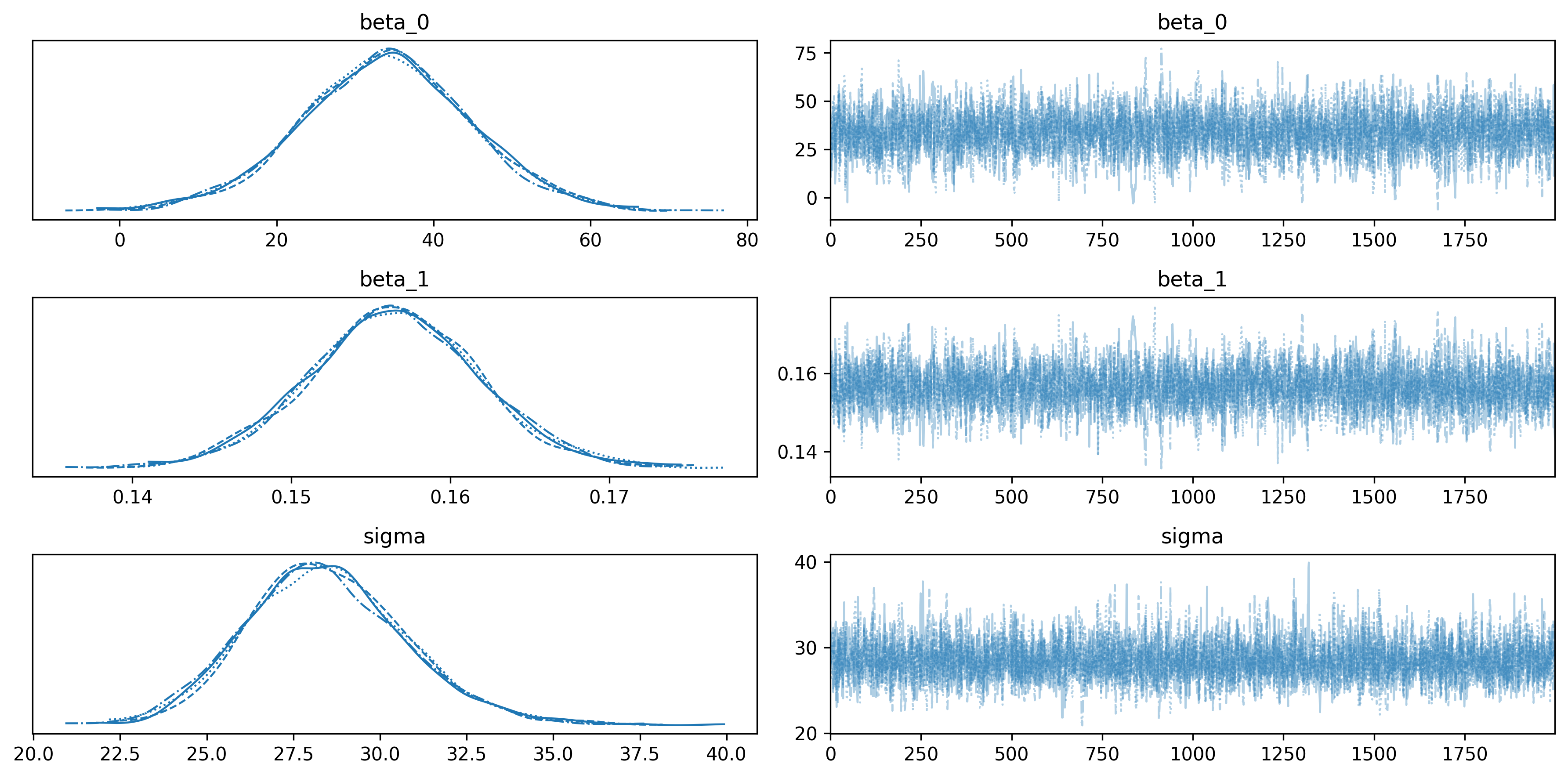
Figure 3.2: Trace plots for the Bayesian linear model. Left: posterior distributions. Right: MCMC chains (should look like fuzzy caterpillars).
The trace plots on the right should look like “fuzzy caterpillars” — all four chains mixing well, with no trends or stuck regions. The density plots on the left show the marginal posterior for each parameter.
Check two numbers in the summary table: r_hat should be 1.00 (all chains agree), and ess_bulk should be well above 400 (enough effective samples for reliable estimates). If either looks off, you need to run the sampler longer or rethink the model.
3.4 Comparing Frequentist and Bayesian Results
Now for the moment of truth. Let us put the OLS estimates and the Bayesian posterior means side by side.
They should be nearly identical. With weakly informative priors and enough data, Bayesian estimation converges to the maximum likelihood estimate — which, for normal errors, is exactly OLS.
A quick sanity check for any Bayesian model
Chris Fonnesbeck offers a simple diagnostic: “The posterior should sit between the prior and the likelihood — if it does not, check your model.” For our linear model, the posterior means land between the prior means (zero, from our weakly informative priors) and the maximum likelihood estimates (the OLS values). Because the priors are wide and the data are plentiful, the posterior is pulled almost entirely toward the data. If the posterior were outside the range spanned by the prior and the likelihood — for instance, farther from zero than the OLS estimate despite a prior centred at zero — that would signal a coding error or a misspecified model. Get in the habit of checking this before interpreting results.
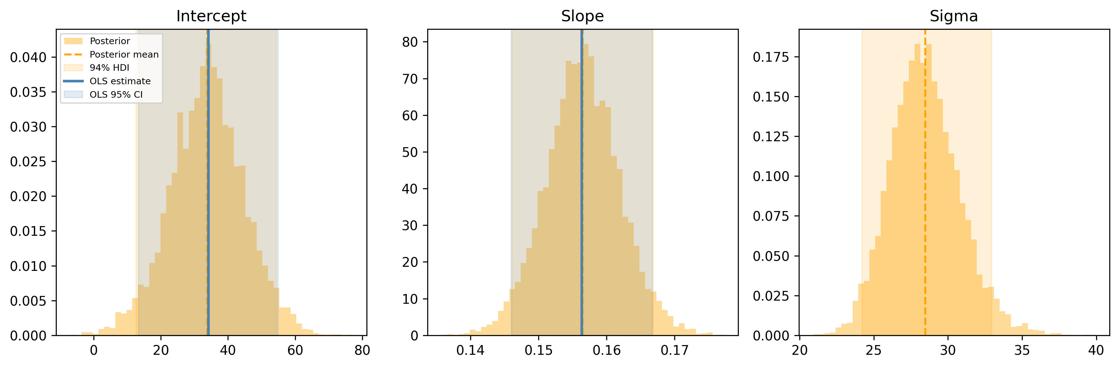
But the Bayesian version gives you something OLS does not (at least not as naturally): the full posterior distribution, not just point estimates. Let us compare the confidence intervals from OLS with the Highest Density Intervals (HDIs) from the posterior:
Figure 3.3: OLS confidence intervals (blue) vs. Bayesian 94% HDIs (orange) for each parameter.
For the intercept and slope, the blue (OLS) and orange (Bayesian) intervals overlap almost perfectly. That is reassuring. The two approaches agree when the problem is well-behaved. The Bayesian version also gives you a posterior for \(\sigma\), which OLS treats as a nuisance parameter you have to extract separately.
3.5 Why Bother Being Bayesian for Linear Regression?
If the answers are the same, why go through the trouble of priors and MCMC? Because the answers are the same only for simple, clean problems. The Bayesian framework pays off when things get messy:
1. Regularization via priors. Setting a tighter prior on \(\beta\) is mathematically equivalent to Ridge regression. A \(\mathcal{N}(0,
\tau^2)\) prior on the coefficients adds an \(L_2\) penalty of strength \(\sigma^2 / \tau^2\). But unlike Ridge, you do not need to tune a regularization hyperparameter — the data determine how much the prior should be trusted.
2. Full uncertainty propagation. When you predict a new observation, the Bayesian model propagates uncertainty through the entire chain: uncertainty in \(\beta_0\), in \(\beta_1\), in \(\sigma\), and the observation noise. OLS prediction intervals approximate this, but the Bayesian version handles it exactly even for small samples and nonlinear transformations.
3. Natural handling of small samples. With 10 data points, OLS confidence intervals rely on asymptotic approximations that may not hold. The Bayesian posterior is exact (given the model). Informative priors can stabilize estimates when data are scarce.
4. Easy extension to hierarchical models. Once you have a Bayesian linear model, adding group structure (different slopes for different cities, different intercepts for different products) is a matter of adding one more level of priors. We will see this in ?sec-hierarchical.
5. Robust alternatives. Replacing the Normal likelihood with a Student-\(t\) makes the model robust to outliers. In OLS, you would need to detect and remove outliers manually. In the Bayesian version, you swap one line of code.
The point is not that Bayesian linear regression is better than OLS for textbook problems. It is that the Bayesian framework is a superset: everything OLS can do, Bayesian regression can do too — and it extends gracefully to problems where OLS breaks down.
3.6 Multiple Regression
Real models have more than one predictor. Let us add a second feature — number of bedrooms — and see how the PyMC model scales.
Before fitting, center and scale the predictors. This is not just good practice — it materially helps the MCMC sampler. When predictors are on different scales (square footage in the thousands, bedrooms in single digits), the posterior geometry becomes an elongated, tilted ellipse. The sampler has to take tiny steps to navigate it, leading to slow mixing and high autocorrelation.
Standardizing the predictors makes the posterior more spherical, which lets the sampler take bigger steps and explore efficiently.
Because the predictors are standardized, the coefficient magnitudes are directly comparable: a one-standard-deviation increase in square footage vs. a one-standard-deviation increase in bedrooms. To recover the coefficients on the original scale, back-transform: \(\beta_{\text{orig}} = \beta_{\text{std}} / \text{sd}(x)\).
post = trace_multi.posteriorslope_sqft_orig = post["beta_sqft"] / sqft_sdslope_bed_orig = post["beta_bed"] / bed_sdprint(f"Slope (sqft), original scale: "f"{float(slope_sqft_orig.mean()):.4f}")print(f"Slope (bedrooms), original scale: "f"{float(slope_bed_orig.mean()):.2f}")print(f"True slope (sqft): {true_slope}")print(f"True slope (bedrooms): {true_beta_bed}")
Slope (sqft), original scale:    0.1504
Slope (bedrooms), original scale: 24.12
True slope (sqft):                0.15
True slope (bedrooms):            20.0
The pattern for adding more predictors is the same: add a prior, add a term to \(\mu\). The model scales linearly with the number of features.
3.7 Bayesian Logistic Regression
Not all outcomes are continuous. When the response is binary — yes/no, click/no-click, survived/died — we need logistic regression. If you have used scikit-learn’s LogisticRegression, you have already fit this model. The idea is the same as linear regression: a linear combination of predictors determines the outcome. But the outcome is a probability bounded between 0 and 1, so we pass the linear combination through the logistic (sigmoid) function:
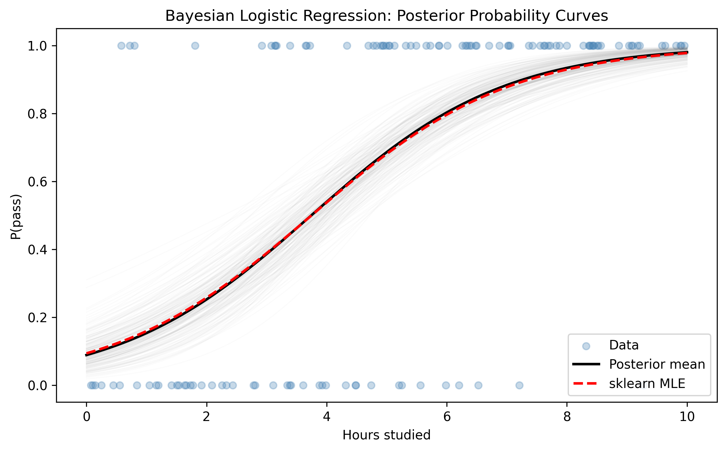
Figure 3.4: Bayesian posterior over the probability curve (gray lines = posterior samples, black = posterior mean). Red dashed = sklearn point estimate.
The gray spaghetti of posterior samples shows the uncertainty in the probability curve. Where data are sparse (very low or very high hours), the curves fan out — the model is less sure. Where data are plentiful, they converge. The sklearn point estimate (red dashed) sits right in the middle. Again: same answer, but the Bayesian version tells you how much to trust it.
This spaghetti plot is one of the most useful visualizations in Bayesian analysis. Every gray line represents one plausible logistic curve drawn from the posterior. A tight bundle of lines means the model is confident; a wide fan means it is not. For a decision-maker — say, a university administrator deciding how many study hours to recommend — the spread of those curves is just as important as their center. The frequentist approach gives you a single curve and a confidence interval table. The Bayesian approach gives you a picture you can look at and immediately understand.
3.8 Robust Regression
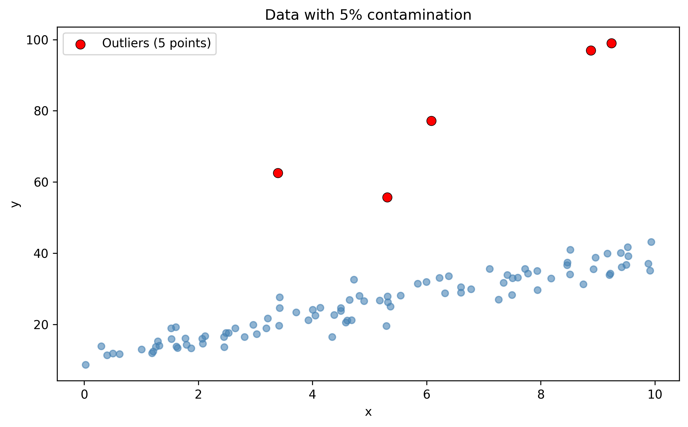
Real-world data have outliers. OLS treats every residual equally, so a single extreme point can drag the entire regression line. The classic frequentist fix is to detect outliers (Cook’s distance, studentized residuals) and remove them. The Bayesian fix is more elegant: replace the Normal likelihood with a Student-\(t\) distribution.
The Student-\(t\) has heavier tails than the Normal. That means it assigns more probability to extreme values, so outliers are “expected” by the model rather than treated as anomalies. The key parameter is the degrees of freedom \(\nu\): small \(\nu\) means heavy tails (robust); as \(\nu \to \infty\), the \(t\) converges to the Normal.
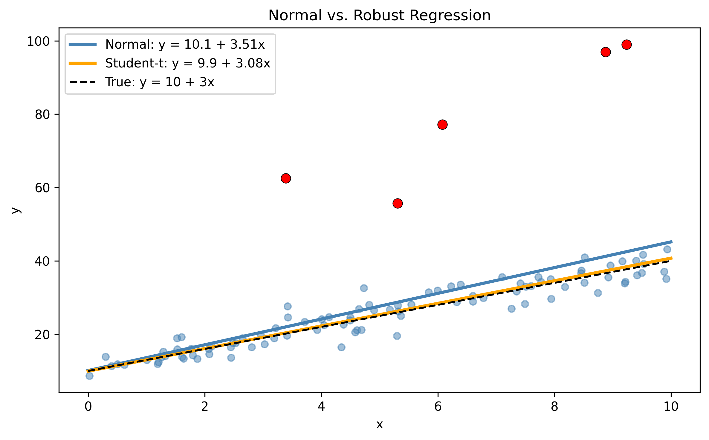
Figure 3.5: Normal vs. Student-t regression on contaminated data. The robust model (orange) is less influenced by the outliers.
The Normal model (blue) gets pulled toward the outliers — both the slope and intercept are biased. The Student-\(t\) model (orange) shrugs off the contamination and recovers a line much closer to the truth (black dashed). The only change was swapping pm.Normal for pm.StudentT and adding a prior on \(\nu\). One line of code buys you robustness that would take pages of diagnostics in the frequentist approach.
This is worth pausing on, because it illustrates a broader principle. In classical statistics, robustness is achieved by detecting and removing problematic observations — a two-step process that requires judgment calls about which points to exclude. In Bayesian modeling, robustness is achieved by choosing a better model — one that accounts for the possibility of extreme values from the start. The outliers are not removed; they are simply given less influence because the model expects them. This is a fundamentally different philosophy: instead of cleaning data to fit the model, you adjust the model to fit the data.
Why heavy tails matter: a lesson from finance
Thomas Wiecki puts it bluntly: “The Normal distribution assumes 2008-scale crashes never happen; the Student-\(t\) is more honest.” Under a Gaussian likelihood, a six-sigma event has a probability on the order of \(10^{-9}\). In financial data, such events happen every few years. The Normal model is not just slightly wrong — it is systematically blind to the most consequential observations.
The practical advice is simple: whenever your data could plausibly contain extreme values — financial returns, insurance claims, network traffic, sensor readings in harsh environments — default to a heavy-tailed likelihood. The Student-\(t\) with a learned \(\nu\) is the easiest upgrade: if the data are well behaved, \(\nu\) will be estimated large and the model reduces to a Normal. If the data have genuine heavy tails, \(\nu\) shrinks and the model accommodates them. You pay almost nothing for this insurance.
Let us check the inferred degrees of freedom:
nu_samples = trace_robust.posterior["nu"].values.flatten()print(f"Posterior mean of nu: {nu_samples.mean():.1f}")print(f"94% HDI of nu: [{np.percentile(nu_samples, 3):.1f}, "f"{np.percentile(nu_samples, 97):.1f}]")
Posterior mean of nu: 1.4
94% HDI of nu: [1.0, 2.1]
A small \(\nu\) (say, below 10) tells you the model found evidence of heavy tails — meaning the outliers are real, not just quirks of the Normal assumption. A large \(\nu\) (above 30) means the data are well-behaved and the \(t\) is essentially acting like a Normal.
3.9 Prediction with Uncertainty
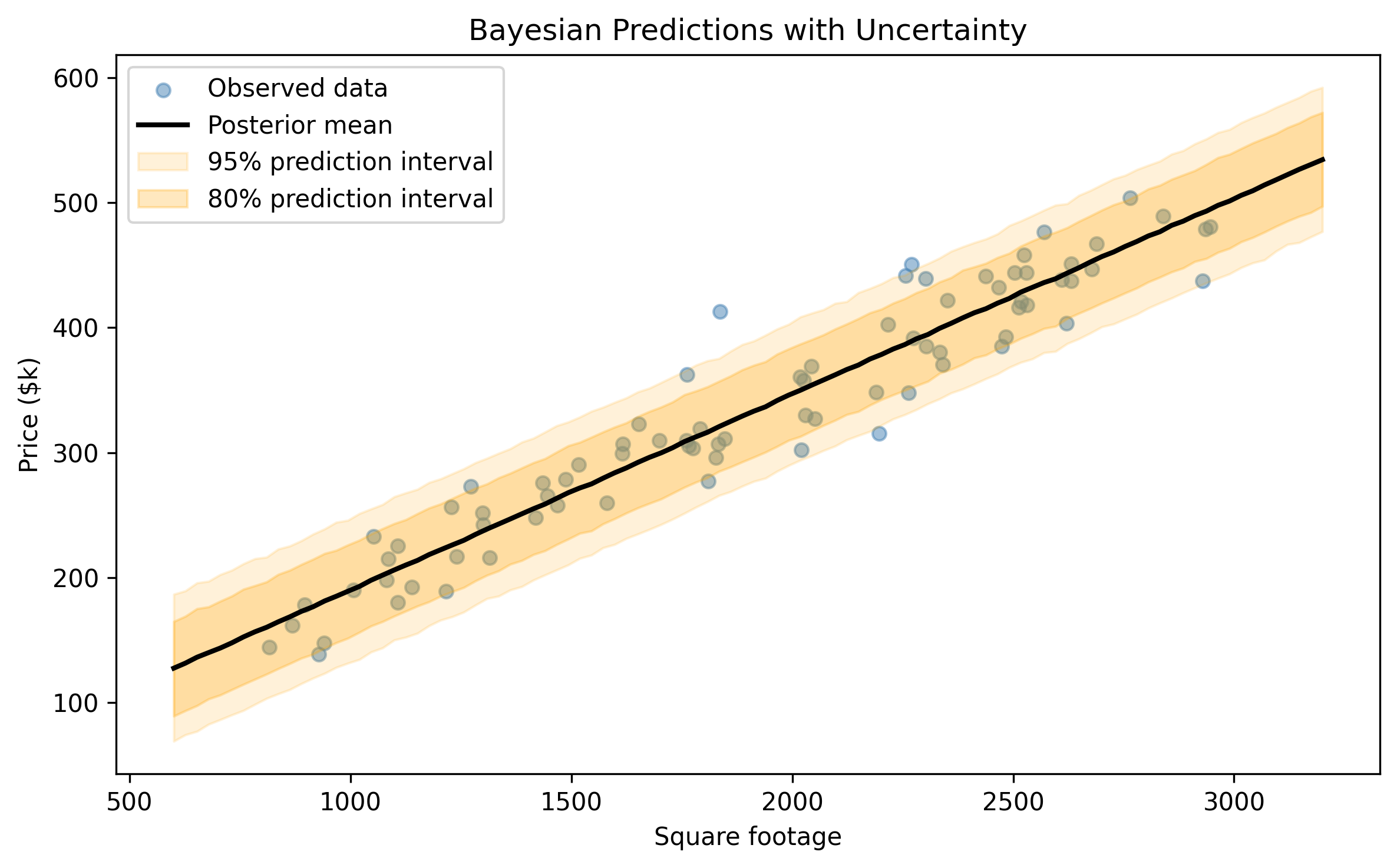
One of the most practical things you can do with a Bayesian model is make predictions that carry uncertainty. Not “the predicted price is $350k” but “the predicted price is $350k, with a 95% chance of being between $290k and $410k.”
PyMC provides pm.sample_posterior_predictive() for exactly this. It takes each posterior draw of the parameters, plugs them into the likelihood, and generates a simulated \(y\) value. The result is the posterior predictive distribution: the full distribution of outcomes you might see for new data, given everything the model has learned.
# Predict on a grid of new sqft values using the simple modelsqft_new = np.linspace(600, 3200, 100)# Use the already-fitted trace to generate predictions# by computing mu and adding noise from the posteriorbeta_0_s = trace.posterior["beta_0"].values.flatten()beta_1_s = trace.posterior["beta_1"].values.flatten()sigma_s = trace.posterior["sigma"].values.flatten()# For each posterior sample, compute predicted y at new sqfty_pred_all = np.zeros((len(beta_0_s), len(sqft_new)))for i inrange(len(beta_0_s)): mu_i = beta_0_s[i] + beta_1_s[i] * sqft_new y_pred_all[i] = rng.normal(mu_i, sigma_s[i])
Figure 3.6: Posterior predictive distribution: the shaded band shows the 95% prediction interval, accounting for both parameter uncertainty and observation noise.
Notice two sources of uncertainty in the prediction band:
Parameter uncertainty — we are not sure exactly where the regression line sits (this is the uncertainty in \(\beta_0\) and \(\beta_1\)).
Observation noise — even if we knew the line perfectly, new observations scatter around it according to \(\sigma\).
The posterior predictive distribution captures both. OLS prediction intervals do something similar, but they rely on normality assumptions and large-sample approximations. The Bayesian version works exactly the same way whether you have 10 observations or 10,000.
In practice, posterior predictive checks are also a powerful model diagnostic. If your prediction intervals are too narrow (real data falls outside them too often), the model is overconfident — maybe you need heavier tails or more predictors. If the intervals are too wide, the model is not learning enough from the data — maybe your priors are too strong or you are missing a key feature. We will return to this idea in ?sec-bayesian-workflow.
3.10 Exercises
Work through these exercises to solidify your understanding. Solutions are provided below each exercise block.
3.10.1 Exercise 1: Prior sensitivity
Refit the simple linear model from ?sec-building-it-in-pymc with a much tighter prior on the slope: pm.Normal("beta_1", mu=0, sigma=0.01). Compare the posterior mean for \(\beta_1\) to the OLS estimate. What happened, and why?
The tight prior pulls \(\beta_1\) toward zero. With \(\sigma = 0.01\), the prior says “I am 95% sure the slope is between \(-0.02\) and \(0.02\).” The data disagree (the true slope is 0.15), but the prior is so strong that the posterior compromises. This is prior-data conflict — the prior overwhelms the evidence. The lesson: wide priors let the data speak; narrow priors encode strong beliefs that had better be right.
3.10.2 Exercise 2: Poisson regression
Fit a Bayesian Poisson regression to model the number of bedrooms as a function of square footage. Use pm.Poisson for the likelihood and a log link: \(\log(\lambda_i) = \beta_0 + \beta_1 x_i\). Does larger square footage predict more bedrooms?
If the HDI for \(\beta_1\) excludes zero, larger square footage is associated with more bedrooms (as we would expect). The Poisson likelihood naturally handles count data — no need to pretend bedrooms are continuous.
3.10.3 Exercise 3: Model comparison
Fit both the Normal and Student-\(t\) models to the clean data (without outliers) from the robust regression section. Use az.compare() with WAIC or LOO to compare them. Which model is preferred when there are no outliers, and why?
When the data are clean, the Normal model should be preferred (or the two should be nearly tied). The Student-\(t\) model has an extra parameter (\(\nu\)) that does not help when there are no outliers, so it gets penalized for complexity. This is the principle of parsimony at work: do not add flexibility you do not need.
3.10.4 Exercise 4: Predict a new house
Using the simple Bayesian linear model, predict the price of a 2000 square-foot house. Report the posterior predictive mean and the 94% HDI of the prediction.
Solution
# Predict for a single house using posterior samplessqft_single =2000.0mu_new = beta_0_s + beta_1_s * sqft_singley_new = rng.normal(mu_new, sigma_s)print(f"Predicted price for 2000 sqft house:")print(f" Posterior predictive mean: ${y_new.mean():.1f}k")hdi_94 = az.hdi(y_new, hdi_prob=0.94)print(f" 94% HDI: [${hdi_94[0]:.1f}k, ${hdi_94[1]:.1f}k]")print(f" True expected price: "f"${true_intercept + true_slope *2000:.1f}k")
The posterior predictive mean should be close to the true expected value of \(50 + 0.15 \times 2000 = 350\). The 94% HDI captures the range of plausible prices, reflecting both parameter uncertainty and observation noise. This is the Bayesian answer to “what price should I expect?” — a full distribution, not a single number.
3.11 Summary
This chapter covered a lot of ground, but the core message is simple. The Bayesian linear model is the same linear model you already know, dressed up with priors and solved with MCMC instead of algebra. For clean data with enough observations, the Bayesian and frequentist answers agree. The Bayesian version earns its keep when you need robustness (Student-\(t\)), uncertainty propagation (posterior predictive), regularization (informative priors), or extensibility (hierarchical models in the next chapter).
The pattern you learned here — define priors, write the likelihood, sample, check diagnostics, interpret — is the same pattern for every PyMC model in this book. The models get more complex; the workflow does not.
Source Code
# Linear Models: From Frequentist to Bayesian```{python}#| echo: falseimport warningswarnings.filterwarnings("ignore", category=FutureWarning)warnings.filterwarnings("ignore", category=UserWarning)```You already know linear regression. Or you did, once. You learned$y = X\beta + \varepsilon$ in a statistics class, ran it in Excel orPython, got a table of coefficients and $p$-values, and moved on. Thatknowledge is the foundation for everything in this chapter.What we are going to do here is take that familiar model and rebuild itas a Bayesian model in PyMC. You will see that the *answers* barelychange --- the posterior means will land right on top of the OLS estimates.But the *questions* you can ask become richer. Instead of a single best-fitline, you get a distribution over regression lines. Instead of confidenceintervals derived from asymptotic theory, you get the full posterioruncertainty over every parameter. And instead of a framework thatstruggles with outliers, missing data, and small samples, you get onethat handles them naturally.The payoff is not dramatic for simple problems. That is the point.Start where the answers are easy to verify, so you can trust themachinery when the problems get hard.## OLS RefresherLinear regression models the relationship between a response variable$y$ and one or more predictors $X$ as:$$y = X\beta + \varepsilon, \qquad \varepsilon \sim \mathcal{N}(0, \sigma^2 I)$$The Ordinary Least Squares (OLS) estimator finds the $\hat{\beta}$ thatminimizes the sum of squared residuals. In matrix form, the closed-formsolution is $\hat{\beta} = (X^\top X)^{-1} X^\top y$. No iteration, notuning --- plug in the data and out comes an answer. That simplicity iswhat makes OLS the workhorse of applied statistics.But notice the assumptions baked into that formula. The errors$\varepsilon$ are normally distributed, have constant variance(homoscedasticity), and are independent of each other. When theseassumptions hold, OLS is hard to beat. When they break down --- outliers,heteroscedasticity, correlated errors, small samples --- the guaranteesevaporate. Keep that in mind as we move through the chapter.Statsmodels gives you OLS in a few lines. Let us generate some datawe can use throughout the chapter. We will simulate a simplerelationship: house price (in thousands of dollars) as a function ofsquare footage, with Gaussian noise.```{python}#| label: ols-dataimport numpy as npimport pandas as pdimport matplotlib.pyplot as pltimport statsmodels.api as smrng = np.random.default_rng(42)# Simulate data: price = 50 + 0.15 * sqft + noisen =80sqft = rng.uniform(800, 3000, size=n)true_intercept =50.0true_slope =0.15noise_sd =30.0price = true_intercept + true_slope * sqft + rng.normal(0, noise_sd, size=n)df = pd.DataFrame({"sqft": sqft, "price": price})df.head()```Now fit OLS with statsmodels:```{python}#| label: ols-fitX_ols = sm.add_constant(df["sqft"])ols_model = sm.OLS(df["price"], X_ols).fit()print(ols_model.summary())```The summary gives you point estimates for the intercept and slope, theirstandard errors, $t$-statistics, $p$-values, and 95% confidenceintervals. For this clean, well-behaved data, OLS works perfectly. Theestimates should land close to the true values we used to generate thedata ($\beta_0 = 50$, $\beta_1 = 0.15$, $\sigma = 30$).Let us visualize the fit:```{python}#| label: fig-ols-fit#| fig-cap: "OLS regression line with 95% confidence band."fig, ax = plt.subplots(figsize=(8, 5))ax.scatter(df["sqft"], df["price"], alpha=0.5, s=30, color="steelblue")x_grid = np.linspace(700, 3100, 200)X_pred = sm.add_constant(x_grid)pred = ols_model.get_prediction(X_pred)pred_summary = pred.summary_frame(alpha=0.05)ax.plot(x_grid, pred_summary["mean"], color="black", linewidth=2)ax.fill_between( x_grid, pred_summary["obs_ci_lower"], pred_summary["obs_ci_upper"], alpha=0.15, color="steelblue", label="95% prediction interval",)ax.fill_between( x_grid, pred_summary["mean_ci_lower"], pred_summary["mean_ci_upper"], alpha=0.3, color="steelblue", label="95% confidence interval",)ax.set_xlabel("Square footage")ax.set_ylabel("Price ($k)")ax.set_title("OLS fit: Price vs. Square Footage")ax.legend(loc="upper left")plt.tight_layout()plt.show()```This is the baseline. Everything that follows should reproduce theseresults --- and then go beyond them.Take a moment to notice what OLS gives you: a single best-fit line, atable of standard errors derived from the residual variance, andconfidence intervals computed from the $t$-distribution. These are all*functions of the data and the model assumptions*. If the assumptionshold, they are exactly right. If they do not, you have no easy way toknow how far off they are. The Bayesian approach will give us adifferent way to think about these same quantities.## The Bayesian Linear ModelThe Bayesian version of linear regression uses the same likelihood:$$y_i \sim \mathcal{N}(\beta_0 + \beta_1 x_i,\; \sigma^2)$$The difference is that we place **prior distributions** on the unknownparameters $\beta_0$, $\beta_1$, and $\sigma$. Instead of computing asingle point estimate, Bayes' theorem gives us a **posteriordistribution** over all three parameters simultaneously:$$p(\beta_0, \beta_1, \sigma \mid y, X) \propto p(y \mid X, \beta_0, \beta_1, \sigma) \; p(\beta_0) \; p(\beta_1) \; p(\sigma)$$Think of it this way. OLS draws *one* line through the data --- the linethat minimizes squared error. The Bayesian model draws *many* lines,each weighted by how well it explains the data and how plausible it isunder the priors. The posterior is the full collection of plausibleregression lines, not just the single best one.For weakly informative priors --- priors that rule out absurd values butdo not strongly favor any particular answer --- the posterior will benearly identical to the OLS result. That is not a bug. It is a sanitycheck. The priors are doing their job: letting the data speak whilegently constraining the model to reasonable territory.Here is the generative model as a plate diagram:$$\boxed{\begin{aligned}\beta_0 &\sim \mathcal{N}(0, 200) \\\beta_1 &\sim \mathcal{N}(0, 10) \\\sigma &\sim \text{HalfNormal}(50) \\\mu_i &= \beta_0 + \beta_1 \, x_i \\y_i &\sim \mathcal{N}(\mu_i, \sigma) \quad \text{for } i = 1, \ldots, n\end{aligned}}$$Each prior says: "I do not know the exact value, but I can rule outvalues that are physically nonsensical." The normal priors on$\beta_0$ and $\beta_1$ are centered at zero with wide standarddeviations. The half-normal prior on $\sigma$ forces the noise scaleto be positive. These are not strong opinions --- they are guardrails.A common worry at this stage is: "Am I not biasing the results bychoosing priors?" With weakly informative priors like these, the answeris *barely*. The prior $\mathcal{N}(0, 200)$ on the intercept says theintercept is somewhere between roughly $-400$ and $400$ --- hardly acontroversial claim for house prices in the hundreds of thousands. Thedata will overwhelm these priors. If you picked a prior of$\mathcal{N}(0, 0.01)$, *that* would bias the results. The distinctionbetween "weakly informative" and "informative" priors is one of the mostimportant practical skills in Bayesian modeling, and we will explore itdirectly in Exercise 1.## Building It in PyMCNow we translate that generative model into PyMC code. Every linemaps directly to a line in the math above.```{python}#| label: pymc-modelimport pymc as pmimport arviz as azwith pm.Model() as linear_model:# Priors beta_0 = pm.Normal("beta_0", mu=0, sigma=200) beta_1 = pm.Normal("beta_1", mu=0, sigma=10) sigma = pm.HalfNormal("sigma", sigma=50)# Expected value mu = beta_0 + beta_1 * df["sqft"].values# Likelihood y_obs = pm.Normal("y_obs", mu=mu, sigma=sigma, observed=df["price"].values, )# Sample from the posterior trace = pm.sample( draws=2000, tune=1000, chains=4, random_seed=42, progressbar=True, )```Let us walk through each piece:- `pm.Normal("beta_0", mu=0, sigma=200)` creates a random variable named `beta_0` with a normal prior. The wide standard deviation of 200 means we are not strongly opinionated about the intercept.- `pm.HalfNormal("sigma", sigma=50)` creates a positive-valued random variable for the noise scale. `HalfNormal` is a normal distribution folded at zero --- it only takes positive values, which is exactly what a standard deviation must be.- `mu = beta_0 + beta_1 * df["sqft"].values` is a deterministic transformation. PyMC tracks this computation through its graph, so the sampler knows how $\mu$ depends on $\beta_0$ and $\beta_1$.- `pm.Normal("y_obs", ..., observed=df["price"].values)` is the likelihood. The `observed` keyword pins this distribution to the actual data. This is what connects the model to reality.- `pm.sample()` runs the MCMC sampler (NUTS, by default) to draw samples from the posterior distribution. We draw 2000 samples per chain across 4 chains, giving us 8000 posterior draws in total.Now check the diagnostics:```{python}#| label: fig-trace#| fig-cap: "Trace plots for the Bayesian linear model. Left: posterior distributions. Right: MCMC chains (should look like fuzzy caterpillars)."az.plot_trace(trace, var_names=["beta_0", "beta_1", "sigma"])plt.tight_layout()plt.show()```The trace plots on the right should look like "fuzzy caterpillars" ---all four chains mixing well, with no trends or stuck regions. Thedensity plots on the left show the marginal posterior for eachparameter.```{python}#| label: posterior-summaryaz.summary(trace, var_names=["beta_0", "beta_1", "sigma"])```Check two numbers in the summary table: `r_hat` should be 1.00 (allchains agree), and `ess_bulk` should be well above 400 (enougheffective samples for reliable estimates). If either looks off, youneed to run the sampler longer or rethink the model.## Comparing Frequentist and Bayesian ResultsNow for the moment of truth. Let us put the OLS estimates and theBayesian posterior means side by side.```{python}#| label: comparison-tableposterior = trace.posteriorbayes_beta0 =float(posterior["beta_0"].mean())bayes_beta1 =float(posterior["beta_1"].mean())bayes_sigma =float(posterior["sigma"].mean())ols_beta0 = ols_model.params[0]ols_beta1 = ols_model.params[1]ols_sigma = np.sqrt(ols_model.mse_resid)comparison = pd.DataFrame({"Parameter": ["Intercept (beta_0)", "Slope (beta_1)", "Sigma"],"True Value": [true_intercept, true_slope, noise_sd],"OLS Estimate": [f"{ols_beta0:.3f}",f"{ols_beta1:.4f}",f"{ols_sigma:.3f}", ],"Bayesian Posterior Mean": [f"{bayes_beta0:.3f}",f"{bayes_beta1:.4f}",f"{bayes_sigma:.3f}", ],})comparison```They should be nearly identical. With weakly informative priors andenough data, Bayesian estimation converges to the maximum likelihoodestimate --- which, for normal errors, is exactly OLS.::: {.callout-tip}## A quick sanity check for any Bayesian modelChris Fonnesbeck offers a simple diagnostic: "The posteriorshould sit between the prior and the likelihood --- if it doesnot, check your model." For our linear model, the posteriormeans land between the prior means (zero, from our weaklyinformative priors) and the maximum likelihood estimates (theOLS values). Because the priors are wide and the data areplentiful, the posterior is pulled almost entirely toward thedata. If the posterior were *outside* the range spanned by theprior and the likelihood --- for instance, farther from zerothan the OLS estimate despite a prior centred at zero --- thatwould signal a coding error or a misspecified model. Get in thehabit of checking this before interpreting results.:::But the Bayesian version gives you something OLS does not (at leastnot as naturally): the **full posterior distribution**, not just pointestimates. Let us compare the confidence intervals from OLS with the**Highest Density Intervals** (HDIs) from the posterior:```{python}#| label: fig-ci-vs-hdi#| fig-cap: "OLS confidence intervals (blue) vs. Bayesian 94% HDIs (orange) for each parameter."fig, axes = plt.subplots(1, 3, figsize=(12, 4))params = ["beta_0", "beta_1", "sigma"]ols_params = [ols_beta0, ols_beta1, ols_sigma]ols_se = [ols_model.bse[0], ols_model.bse[1], None]titles = ["Intercept", "Slope", "Sigma"]for i, (pname, title) inenumerate(zip(params, titles)): ax = axes[i]# Bayesian HDI samples = posterior[pname].values.flatten() hdi = az.hdi(trace, var_names=[pname], hdi_prob=0.94) hdi_vals = hdi[pname].values ax.hist( samples, bins=50, density=True, alpha=0.4, color="orange", label="Posterior", ) ax.axvline(float(np.mean(samples)), color="orange", linestyle="--", linewidth=1.5, label="Posterior mean", ) ax.axvspan( hdi_vals[0], hdi_vals[1], alpha=0.15, color="orange", label="94% HDI", )# OLS point estimate and CI (for beta_0 and beta_1)if ols_se[i] isnotNone: ax.axvline( ols_params[i], color="steelblue", linestyle="-", linewidth=2, label="OLS estimate", ) ci_low = ols_params[i] -1.96* ols_se[i] ci_high = ols_params[i] +1.96* ols_se[i] ax.axvspan( ci_low, ci_high, alpha=0.15, color="steelblue", label="OLS 95% CI", ) ax.set_title(title)if i ==0: ax.legend(fontsize=7, loc="upper left")plt.tight_layout()plt.show()```For the intercept and slope, the blue (OLS) and orange (Bayesian)intervals overlap almost perfectly. That is reassuring. The twoapproaches agree when the problem is well-behaved. The Bayesian versionalso gives you a posterior for $\sigma$, which OLS treats as a nuisanceparameter you have to extract separately.## Why Bother Being Bayesian for Linear Regression?If the answers are the same, why go through the trouble of priors andMCMC? Because the answers are the same *only* for simple, cleanproblems. The Bayesian framework pays off when things get messy:**1. Regularization via priors.** Setting a tighter prior on $\beta$ ismathematically equivalent to Ridge regression. A $\mathcal{N}(0,\tau^2)$ prior on the coefficients adds an $L_2$ penalty of strength$\sigma^2 / \tau^2$. But unlike Ridge, you do not need to tune aregularization hyperparameter --- the data determine how much the priorshould be trusted.**2. Full uncertainty propagation.** When you predict a new observation,the Bayesian model propagates uncertainty through the entire chain:uncertainty in $\beta_0$, in $\beta_1$, in $\sigma$, and theobservation noise. OLS prediction intervals approximate this, but theBayesian version handles it exactly even for small samples andnonlinear transformations.**3. Natural handling of small samples.** With 10 data points, OLSconfidence intervals rely on asymptotic approximations that may nothold. The Bayesian posterior is exact (given the model). Informativepriors can stabilize estimates when data are scarce.**4. Easy extension to hierarchical models.** Once you have a Bayesianlinear model, adding group structure (different slopes for differentcities, different intercepts for different products) is a matter ofadding one more level of priors. We will see this in @sec-hierarchical.**5. Robust alternatives.** Replacing the Normal likelihood with aStudent-$t$ makes the model robust to outliers. In OLS, you would needto detect and remove outliers manually. In the Bayesian version, youswap one line of code.The point is not that Bayesian linear regression is better than OLS fortextbook problems. It is that the Bayesian framework is a *superset*:everything OLS can do, Bayesian regression can do too --- and it extendsgracefully to problems where OLS breaks down.## Multiple RegressionReal models have more than one predictor. Let us add a second feature--- number of bedrooms --- and see how the PyMC model scales.```{python}#| label: multi-data# Add bedrooms as a second predictorbedrooms = rng.poisson(lam=2, size=n) +1# 1-6 bedroomstrue_beta_bed =20.0price_multi = ( true_intercept+ true_slope * sqft+ true_beta_bed * bedrooms+ rng.normal(0, noise_sd, size=n))df_multi = pd.DataFrame({"sqft": sqft,"bedrooms": bedrooms,"price": price_multi,})df_multi.head()```### Why centering and scaling helps MCMCBefore fitting, center and scale the predictors. This is not just goodpractice --- it materially helps the MCMC sampler. When predictors are ondifferent scales (square footage in the thousands, bedrooms in singledigits), the posterior geometry becomes an elongated, tilted ellipse.The sampler has to take tiny steps to navigate it, leading to slowmixing and high autocorrelation.Standardizing the predictors makes the posterior more spherical, whichlets the sampler take bigger steps and explore efficiently.```{python}#| label: multi-center# Standardize predictorssqft_mean, sqft_sd = df_multi["sqft"].mean(), df_multi["sqft"].std()bed_mean, bed_sd = df_multi["bedrooms"].mean(), df_multi["bedrooms"].std()sqft_z = (df_multi["sqft"] - sqft_mean) / sqft_sdbed_z = (df_multi["bedrooms"] - bed_mean) / bed_sd``````{python}#| label: multi-modelwith pm.Model() as multi_model:# Priors on standardized scale beta_0 = pm.Normal("beta_0", mu=0, sigma=200) beta_sqft = pm.Normal("beta_sqft", mu=0, sigma=50) beta_bed = pm.Normal("beta_bed", mu=0, sigma=50) sigma = pm.HalfNormal("sigma", sigma=50) mu = beta_0 + beta_sqft * sqft_z.values + beta_bed * bed_z.values y_obs = pm.Normal("y_obs", mu=mu, sigma=sigma, observed=df_multi["price"].values, ) trace_multi = pm.sample( draws=2000, tune=1000, chains=4, random_seed=42, )``````{python}#| label: multi-summaryaz.summary( trace_multi, var_names=["beta_0", "beta_sqft", "beta_bed", "sigma"],)```Because the predictors are standardized, the coefficient magnitudesare directly comparable: a one-standard-deviation increase in squarefootage vs. a one-standard-deviation increase in bedrooms. To recoverthe coefficients on the original scale, back-transform:$\beta_{\text{orig}} = \beta_{\text{std}} / \text{sd}(x)$.```{python}#| label: multi-backtransformpost = trace_multi.posteriorslope_sqft_orig = post["beta_sqft"] / sqft_sdslope_bed_orig = post["beta_bed"] / bed_sdprint(f"Slope (sqft), original scale: "f"{float(slope_sqft_orig.mean()):.4f}")print(f"Slope (bedrooms), original scale: "f"{float(slope_bed_orig.mean()):.2f}")print(f"True slope (sqft): {true_slope}")print(f"True slope (bedrooms): {true_beta_bed}")```The pattern for adding more predictors is the same: add a prior, add aterm to $\mu$. The model scales linearly with the number of features.## Bayesian Logistic RegressionNot all outcomes are continuous. When the response is binary --- yes/no,click/no-click, survived/died --- we need logistic regression. If you haveused scikit-learn's `LogisticRegression`, you have already fit thismodel. The idea is the same as linear regression: a linear combinationof predictors determines the outcome. But the outcome is a probabilitybounded between 0 and 1, so we pass the linear combination through the**logistic (sigmoid) function**:$$p_i = \text{logit}^{-1}(\beta_0 + \beta_1 x_i) = \frac{1}{1 + e^{-(\beta_0 + \beta_1 x_i)}}$$$$y_i \sim \text{Bernoulli}(p_i)$$Let us simulate a dataset where the probability of passing an examdepends on hours of study:```{python}#| label: logistic-data# Simulate logistic data: P(pass) depends on hours studiedn_students =120hours = rng.uniform(0, 10, size=n_students)true_b0_log =-3.0true_b1_log =0.8logit_p = true_b0_log + true_b1_log * hoursprob_pass =1.0/ (1.0+ np.exp(-logit_p))passed = rng.binomial(n=1, p=prob_pass)print(f"Pass rate: {passed.mean():.2%}")``````{python}#| label: logistic-modelwith pm.Model() as logistic_model: b0 = pm.Normal("b0", mu=0, sigma=5) b1 = pm.Normal("b1", mu=0, sigma=5)# Linear predictor passed through sigmoid p = pm.math.sigmoid(b0 + b1 * hours)# Bernoulli likelihood y_obs = pm.Bernoulli("y_obs", p=p, observed=passed) trace_logistic = pm.sample( draws=2000, tune=1000, chains=4, random_seed=42, )``````{python}#| label: logistic-summaryaz.summary(trace_logistic, var_names=["b0", "b1"])```Now compare the Bayesian result to scikit-learn's `LogisticRegression`:```{python}#| label: fig-logistic-compare#| fig-cap: "Bayesian posterior over the probability curve (gray lines = posterior samples, black = posterior mean). Red dashed = sklearn point estimate."from sklearn.linear_model import LogisticRegression# Sklearn fitlr = LogisticRegression(penalty=None, solver="lbfgs")lr.fit(hours.reshape(-1, 1), passed)sk_b0 = lr.intercept_[0]sk_b1 = lr.coef_[0, 0]# Plotfig, ax = plt.subplots(figsize=(8, 5))ax.scatter( hours, passed, alpha=0.3, s=30, color="steelblue", label="Data",)x_grid = np.linspace(0, 10, 200)# Posterior samples of the probability curvepost_log = trace_logistic.posteriorb0_samples = post_log["b0"].values.flatten()b1_samples = post_log["b1"].values.flatten()idx = rng.choice(len(b0_samples), size=200, replace=False)for j in idx: p_curve =1.0/ (1.0+ np.exp(-(b0_samples[j] + b1_samples[j] * x_grid))) ax.plot(x_grid, p_curve, color="gray", alpha=0.03, linewidth=0.8)# Posterior mean curvep_mean =1.0/ (1.0+ np.exp(-(b0_samples.mean() + b1_samples.mean() * x_grid)))ax.plot(x_grid, p_mean, color="black", linewidth=2, label="Posterior mean")# Sklearn curvep_sk =1.0/ (1.0+ np.exp(-(sk_b0 + sk_b1 * x_grid)))ax.plot( x_grid, p_sk, color="red", linewidth=2, linestyle="--", label="sklearn MLE",)ax.set_xlabel("Hours studied")ax.set_ylabel("P(pass)")ax.set_title("Bayesian Logistic Regression: Posterior Probability Curves")ax.legend(loc="lower right")plt.tight_layout()plt.show()```The gray spaghetti of posterior samples shows the *uncertainty* in theprobability curve. Where data are sparse (very low or very high hours),the curves fan out --- the model is less sure. Where data are plentiful,they converge. The sklearn point estimate (red dashed) sits right in themiddle. Again: same answer, but the Bayesian version tells you *how muchto trust it*.This spaghetti plot is one of the most useful visualizations in Bayesiananalysis. Every gray line represents one plausible logistic curve drawnfrom the posterior. A tight bundle of lines means the model is confident;a wide fan means it is not. For a decision-maker --- say, a universityadministrator deciding how many study hours to recommend --- the spreadof those curves is just as important as their center. The frequentistapproach gives you a single curve and a confidence interval table. TheBayesian approach gives you a picture you can *look at* and immediatelyunderstand.## Robust RegressionReal-world data have outliers. OLS treats every residual equally, so asingle extreme point can drag the entire regression line. The classicfrequentist fix is to detect outliers (Cook's distance, studentizedresiduals) and remove them. The Bayesian fix is more elegant: replacethe Normal likelihood with a **Student-$t$ distribution**.The Student-$t$ has heavier tails than the Normal. That means itassigns more probability to extreme values, so outliers are "expected"by the model rather than treated as anomalies. The key parameter is thedegrees of freedom $\nu$: small $\nu$ means heavy tails (robust); as$\nu \to \infty$, the $t$ converges to the Normal.Let us see this in action with contaminated data:```{python}#| label: robust-data# Generate clean data plus 5% contaminationn_robust =100x_robust = rng.uniform(0, 10, size=n_robust)y_clean =10+3* x_robust + rng.normal(0, 3, size=n_robust)# Add 5% outliersn_outliers =int(0.05* n_robust)outlier_idx = rng.choice(n_robust, size=n_outliers, replace=False)y_contaminated = y_clean.copy()y_contaminated[outlier_idx] += rng.uniform(30, 60, size=n_outliers)fig, ax = plt.subplots(figsize=(8, 5))ax.scatter( x_robust, y_contaminated, alpha=0.6, s=30, color="steelblue",)ax.scatter( x_robust[outlier_idx], y_contaminated[outlier_idx], color="red", s=60, zorder=5, label=f"Outliers ({n_outliers} points)", edgecolor="black", linewidth=0.5,)ax.set_xlabel("x")ax.set_ylabel("y")ax.set_title("Data with 5% contamination")ax.legend()plt.tight_layout()plt.show()```Now fit two models --- one with a Normal likelihood, one with aStudent-$t$ likelihood --- and compare:```{python}#| label: robust-models# Model 1: Normal likelihood (sensitive to outliers)with pm.Model() as normal_model: b0 = pm.Normal("b0", mu=0, sigma=50) b1 = pm.Normal("b1", mu=0, sigma=20) sigma = pm.HalfNormal("sigma", sigma=20) mu = b0 + b1 * x_robust y_obs = pm.Normal("y_obs", mu=mu, sigma=sigma, observed=y_contaminated) trace_normal = pm.sample( draws=2000, tune=1000, chains=4, random_seed=42, )# Model 2: Student-t likelihood (robust to outliers)with pm.Model() as robust_model: b0 = pm.Normal("b0", mu=0, sigma=50) b1 = pm.Normal("b1", mu=0, sigma=20) sigma = pm.HalfNormal("sigma", sigma=20) nu = pm.Exponential("nu", lam=1/30) # prior on degrees of freedom mu = b0 + b1 * x_robust y_obs = pm.StudentT("y_obs", nu=nu, mu=mu, sigma=sigma, observed=y_contaminated, ) trace_robust = pm.sample( draws=2000, tune=1000, chains=4, random_seed=42, )``````{python}#| label: fig-robust-compare#| fig-cap: "Normal vs. Student-t regression on contaminated data. The robust model (orange) is less influenced by the outliers."fig, ax = plt.subplots(figsize=(8, 5))ax.scatter( x_robust, y_contaminated, alpha=0.5, s=30, color="steelblue",)ax.scatter( x_robust[outlier_idx], y_contaminated[outlier_idx], color="red", s=60, zorder=5, edgecolor="black", linewidth=0.5,)x_line = np.linspace(0, 10, 200)# Normal model linepost_n = trace_normal.posteriorb0_n =float(post_n["b0"].mean())b1_n =float(post_n["b1"].mean())ax.plot( x_line, b0_n + b1_n * x_line, color="steelblue", linewidth=2.5, label=f"Normal: y = {b0_n:.1f} + {b1_n:.2f}x",)# Robust model linepost_r = trace_robust.posteriorb0_r =float(post_r["b0"].mean())b1_r =float(post_r["b1"].mean())ax.plot( x_line, b0_r + b1_r * x_line, color="orange", linewidth=2.5, label=f"Student-t: y = {b0_r:.1f} + {b1_r:.2f}x",)# True lineax.plot( x_line,10+3* x_line, color="black", linewidth=1.5, linestyle="--", label="True: y = 10 + 3x",)ax.set_xlabel("x")ax.set_ylabel("y")ax.set_title("Normal vs. Robust Regression")ax.legend(loc="upper left")plt.tight_layout()plt.show()```The Normal model (blue) gets pulled toward the outliers --- both theslope and intercept are biased. The Student-$t$ model (orange) shrugsoff the contamination and recovers a line much closer to the truth(black dashed). The only change was swapping `pm.Normal` for`pm.StudentT` and adding a prior on $\nu$. One line of code buys yourobustness that would take pages of diagnostics in the frequentistapproach.This is worth pausing on, because it illustrates a broader principle.In classical statistics, robustness is achieved by *detecting andremoving* problematic observations --- a two-step process that requiresjudgment calls about which points to exclude. In Bayesian modeling,robustness is achieved by *choosing a better model* --- one thataccounts for the possibility of extreme values from the start. Theoutliers are not removed; they are simply given less influence becausethe model expects them. This is a fundamentally different philosophy:instead of cleaning data to fit the model, you adjust the model to fitthe data.::: {.callout-note}## Why heavy tails matter: a lesson from financeThomas Wiecki puts it bluntly: "The Normal distribution assumes2008-scale crashes never happen; the Student-$t$ is more honest."Under a Gaussian likelihood, a six-sigma event has a probabilityon the order of $10^{-9}$. In financial data, such events happenevery few years. The Normal model is not just slightly wrong ---it is *systematically* blind to the most consequentialobservations.The practical advice is simple: whenever your data couldplausibly contain extreme values --- financial returns, insuranceclaims, network traffic, sensor readings in harsh environments--- default to a heavy-tailed likelihood. The Student-$t$ with alearned $\nu$ is the easiest upgrade: if the data are wellbehaved, $\nu$ will be estimated large and the model reduces toa Normal. If the data have genuine heavy tails, $\nu$ shrinksand the model accommodates them. You pay almost nothing for thisinsurance.:::Let us check the inferred degrees of freedom:```{python}#| label: robust-nunu_samples = trace_robust.posterior["nu"].values.flatten()print(f"Posterior mean of nu: {nu_samples.mean():.1f}")print(f"94% HDI of nu: [{np.percentile(nu_samples, 3):.1f}, "f"{np.percentile(nu_samples, 97):.1f}]")```A small $\nu$ (say, below 10) tells you the model found evidence ofheavy tails --- meaning the outliers are real, not just quirks of theNormal assumption. A large $\nu$ (above 30) means the data arewell-behaved and the $t$ is essentially acting like a Normal.## Prediction with UncertaintyOne of the most practical things you can do with a Bayesian model ismake predictions that carry uncertainty. Not "the predicted price is\$350k" but "the predicted price is \$350k, with a 95% chance of beingbetween \$290k and \$410k."PyMC provides `pm.sample_posterior_predictive()` for exactly this. Ittakes each posterior draw of the parameters, plugs them into thelikelihood, and generates a simulated $y$ value. The result is the**posterior predictive distribution**: the full distribution of outcomesyou might see for new data, given everything the model has learned.```{python}#| label: prediction# Predict on a grid of new sqft values using the simple modelsqft_new = np.linspace(600, 3200, 100)# Use the already-fitted trace to generate predictions# by computing mu and adding noise from the posteriorbeta_0_s = trace.posterior["beta_0"].values.flatten()beta_1_s = trace.posterior["beta_1"].values.flatten()sigma_s = trace.posterior["sigma"].values.flatten()# For each posterior sample, compute predicted y at new sqfty_pred_all = np.zeros((len(beta_0_s), len(sqft_new)))for i inrange(len(beta_0_s)): mu_i = beta_0_s[i] + beta_1_s[i] * sqft_new y_pred_all[i] = rng.normal(mu_i, sigma_s[i])``````{python}#| label: fig-prediction#| fig-cap: "Posterior predictive distribution: the shaded band shows the 95% prediction interval, accounting for both parameter uncertainty and observation noise."y_pred = y_pred_allpred_mean = y_pred.mean(axis=0)pred_lower = np.percentile(y_pred, 2.5, axis=0)pred_upper = np.percentile(y_pred, 97.5, axis=0)pred_10 = np.percentile(y_pred, 10, axis=0)pred_90 = np.percentile(y_pred, 90, axis=0)fig, ax = plt.subplots(figsize=(8, 5))ax.scatter( df["sqft"], df["price"], alpha=0.5, s=30, color="steelblue", label="Observed data",)ax.plot( sqft_new, pred_mean, color="black", linewidth=2, label="Posterior mean",)ax.fill_between( sqft_new, pred_lower, pred_upper, alpha=0.15, color="orange", label="95% prediction interval",)ax.fill_between( sqft_new, pred_10, pred_90, alpha=0.25, color="orange", label="80% prediction interval",)ax.set_xlabel("Square footage")ax.set_ylabel("Price ($k)")ax.set_title("Bayesian Predictions with Uncertainty")ax.legend(loc="upper left")plt.tight_layout()plt.show()```Notice two sources of uncertainty in the prediction band:1. **Parameter uncertainty** --- we are not sure exactly where the regression line sits (this is the uncertainty in $\beta_0$ and $\beta_1$).2. **Observation noise** --- even if we knew the line perfectly, new observations scatter around it according to $\sigma$.The posterior predictive distribution captures *both*. OLS predictionintervals do something similar, but they rely on normality assumptionsand large-sample approximations. The Bayesian version works exactly thesame way whether you have 10 observations or 10,000.In practice, posterior predictive checks are also a powerful modeldiagnostic. If your prediction intervals are too narrow (real datafalls outside them too often), the model is overconfident --- maybe youneed heavier tails or more predictors. If the intervals are too wide,the model is not learning enough from the data --- maybe your priors aretoo strong or you are missing a key feature. We will return to thisidea in @sec-bayesian-workflow.## ExercisesWork through these exercises to solidify your understanding. Solutionsare provided below each exercise block.### Exercise 1: Prior sensitivityRefit the simple linear model from @sec-building-it-in-pymc with a*much* tighter prior on the slope: `pm.Normal("beta_1", mu=0,sigma=0.01)`. Compare the posterior mean for $\beta_1$ to the OLSestimate. What happened, and why?::: {.callout-tip collapse="true" title="Solution"}```{python}#| label: ex1-solutionwith pm.Model() as tight_prior_model: beta_0 = pm.Normal("beta_0", mu=0, sigma=200) beta_1 = pm.Normal("beta_1", mu=0, sigma=0.01) # very tight! sigma = pm.HalfNormal("sigma", sigma=50) mu = beta_0 + beta_1 * df["sqft"].values y_obs = pm.Normal("y_obs", mu=mu, sigma=sigma, observed=df["price"].values, ) trace_tight = pm.sample( draws=2000, tune=1000, chains=4, random_seed=42, )post_tight = trace_tight.posteriorprint(f"Tight prior -- beta_1 posterior mean: "f"{float(post_tight['beta_1'].mean()):.6f}")print(f"OLS estimate: "f"{ols_beta1:.6f}")print(f"True value: "f"{true_slope:.6f}")```The tight prior pulls $\beta_1$ toward zero. With $\sigma = 0.01$, theprior says "I am 95% sure the slope is between $-0.02$ and $0.02$."The data disagree (the true slope is 0.15), but the prior is so strongthat the posterior compromises. This is **prior-data conflict** --- theprior overwhelms the evidence. The lesson: wide priors let the dataspeak; narrow priors encode strong beliefs that had better be right.:::### Exercise 2: Poisson regressionFit a Bayesian Poisson regression to model the number of bedrooms as afunction of square footage. Use `pm.Poisson` for the likelihood and alog link: $\log(\lambda_i) = \beta_0 + \beta_1 x_i$. Does largersquare footage predict more bedrooms?::: {.callout-tip collapse="true" title="Solution"}```{python}#| label: ex2-solutionimport pytensor.tensor as ptwith pm.Model() as poisson_model: b0 = pm.Normal("b0", mu=0, sigma=5) b1 = pm.Normal("b1", mu=0, sigma=5)# Standardize sqft for better sampling sqft_std = (df_multi["sqft"].values - sqft_mean) / sqft_sd log_lambda = b0 + b1 * sqft_std lam = pt.exp(log_lambda) y_obs = pm.Poisson("y_obs", mu=lam, observed=df_multi["bedrooms"].values, ) trace_poisson = pm.sample( draws=2000, tune=1000, chains=4, random_seed=42, )print(az.summary(trace_poisson, var_names=["b0", "b1"]))```If the HDI for $\beta_1$ excludes zero, larger square footage isassociated with more bedrooms (as we would expect). The Poissonlikelihood naturally handles count data --- no need to pretendbedrooms are continuous.:::### Exercise 3: Model comparisonFit both the Normal and Student-$t$ models to the *clean* data (withoutoutliers) from the robust regression section. Use `az.compare()` withWAIC or LOO to compare them. Which model is preferred when there are nooutliers, and why?::: {.callout-tip collapse="true" title="Solution"}```{python}#| label: ex3-solution# Fit both models to clean datawith pm.Model() as clean_normal: b0 = pm.Normal("b0", mu=0, sigma=50) b1 = pm.Normal("b1", mu=0, sigma=20) sigma = pm.HalfNormal("sigma", sigma=20) mu = b0 + b1 * x_robust y_obs = pm.Normal("y_obs", mu=mu, sigma=sigma, observed=y_clean) trace_cn = pm.sample( draws=2000, tune=1000, chains=4, random_seed=42, idata_kwargs={"log_likelihood": True}, )with pm.Model() as clean_robust: b0 = pm.Normal("b0", mu=0, sigma=50) b1 = pm.Normal("b1", mu=0, sigma=20) sigma = pm.HalfNormal("sigma", sigma=20) nu = pm.Exponential("nu", lam=1/30) mu = b0 + b1 * x_robust y_obs = pm.StudentT("y_obs", nu=nu, mu=mu, sigma=sigma, observed=y_clean, ) trace_cr = pm.sample( draws=2000, tune=1000, chains=4, random_seed=42, idata_kwargs={"log_likelihood": True}, )comp = az.compare( {"Normal": trace_cn, "Student-t": trace_cr}, ic="loo",)print(comp)```When the data are clean, the Normal model should be preferred (orthe two should be nearly tied). The Student-$t$ model has an extraparameter ($\nu$) that does not help when there are no outliers, soit gets penalized for complexity. This is the principle of parsimonyat work: do not add flexibility you do not need.:::### Exercise 4: Predict a new houseUsing the simple Bayesian linear model, predict the price of a 2000square-foot house. Report the posterior predictive mean and the 94% HDIof the prediction.::: {.callout-tip collapse="true" title="Solution"}```{python}#| label: ex4-solution# Predict for a single house using posterior samplessqft_single =2000.0mu_new = beta_0_s + beta_1_s * sqft_singley_new = rng.normal(mu_new, sigma_s)print(f"Predicted price for 2000 sqft house:")print(f" Posterior predictive mean: ${y_new.mean():.1f}k")hdi_94 = az.hdi(y_new, hdi_prob=0.94)print(f" 94% HDI: [${hdi_94[0]:.1f}k, ${hdi_94[1]:.1f}k]")print(f" True expected price: "f"${true_intercept + true_slope *2000:.1f}k")```The posterior predictive mean should be close to the true expected valueof $50 + 0.15 \times 2000 = 350$. The 94% HDI captures the range ofplausible prices, reflecting both parameter uncertainty and observationnoise. This is the Bayesian answer to "what price should I expect?" ---a full distribution, not a single number.:::## SummaryThis chapter covered a lot of ground, but the core message is simple.The Bayesian linear model is the same linear model you already know,dressed up with priors and solved with MCMC instead of algebra. Forclean data with enough observations, the Bayesian and frequentistanswers agree. The Bayesian version earns its keep when you needrobustness (Student-$t$), uncertainty propagation (posterior predictive),regularization (informative priors), or extensibility (hierarchicalmodels in the next chapter).The pattern you learned here --- define priors, write the likelihood,sample, check diagnostics, interpret --- is the same pattern for everyPyMC model in this book. The models get more complex; the workflow doesnot.