2  PyMC Fundamentals: Model Building and Sampling

In Chapter 1 you learned why Bayesian thinking matters. Now you learn how to do it in code. This chapter introduces PyMC’s core machinery: the model context, distributions, sampling, and diagnostics. By the end you will have built a complete model from scratch, inspected its output, and verified it works.

Everything here generalises. The simple model we build—estimating the mean and spread of normally distributed data—uses the same workflow you will apply to hierarchical models, GLMs, and Gaussian processes in later chapters. Learn this workflow once, and you have learned the skeleton of every PyMC project.

import pymc as pm
import arviz as az
import numpy as np
import matplotlib.pyplot as plt
from numpy.random import default_rng

rng = default_rng(42)
print(f"PyMC version: {pm.__version__}")

PyMC version: 5.25.1

2.1 The PyMC Model Context

Every PyMC model starts the same way:

with pm.Model() as model:
    # define your model here
    ...

This pattern looks like opening a file with with open(...). The analogy is apt. Just as a file context manager handles cleanup when you are done, the model context manager handles bookkeeping. Every random variable you create inside the with block is automatically registered to that model.

Why a context manager? PyMC needs to track which random variables belong together. When you write pm.Normal("mu", mu=0, sigma=1) inside a model context, PyMC records that variable in an internal graph. Later, when you call pm.sample(), PyMC reads that graph and figures out how all the pieces connect. Without the context manager, PyMC would not know which variables belong to your model.

Think of it like a whiteboard. You say “okay, everything I draw on this whiteboard is part of Model A.” Then you sketch your distributions, your data, and your connections. When you step back, PyMC photographs the whiteboard and uses it for inference.

with pm.Model() as demo_model:
    x = pm.Normal("x", mu=0, sigma=1)
    y = pm.Normal("y", mu=x, sigma=0.5)

# The model knows about both variables:
print(demo_model.named_vars.keys())

dict_keys(['x', 'y'])

Two things to notice:

1. Variables have string names. The first argument to any distribution is a name ("x", "y"). This name appears in trace summaries, plots, and diagnostics. Pick descriptive names.
2. Variables can depend on each other. We defined y with mu=x. PyMC records this dependency in its computational graph. During sampling, it respects the relationship.

You can also create a model without the as syntax:

model = pm.Model()
with model:
    ...

Both are equivalent. The as form is more common because it reads naturally.

2.1.1 What Happens Under the Hood

When you create a variable inside the context, PyMC does several things silently:

1. Registers the variable in the model’s variable list.
2. Records its distribution (type, parameters) so the sampler knows the probability of any value.
3. Builds a computational graph (using PyTensor, the tensor library behind PyMC) that connects this variable to others.
4. Assigns a default initial value that the sampler will use as a starting point.

You never need to do any of this manually. The context manager is the glue that makes PyMC feel declarative—you describe the model, and PyMC figures out how to compute with it.

2.1.2 Multiple Models in One Script

You can define multiple models in the same script. Each with pm.Model() block creates an independent model:

with pm.Model() as model_a:
    x = pm.Normal("x", mu=0, sigma=1)

with pm.Model() as model_b:
    x = pm.Normal("x", mu=5, sigma=2)

The two x variables live in different models and do not interact. This is useful when you want to compare alternative model specifications on the same data.

2.1.3 Common Mistakes with the Model Context

Mistake 1: Forgetting the context. If you create a distribution outside any with pm.Model() block, PyMC raises an error. Every distribution needs a home.

Mistake 2: Mixing up models. If you have two models open (which is unusual), variables go to the innermost active context. Keep your model blocks clean and separate.

Mistake 3: Reusing variable names. Within one model, each variable name must be unique. PyMC uses names as dictionary keys. If you accidentally write pm.Normal("mu", ...) twice, you will get an error.

2.2 Distributions in PyMC

Distributions are the building blocks of Bayesian models. Each distribution represents your belief about what values a parameter or observation might take. PyMC provides dozens of distributions. Here are the ones you will use most often.

2.2.1 Continuous Distributions

Distribution	PyMC syntax	Typical use
Normal	pm.Normal("x", mu=0, sigma=1)	Means, regression coefficients
Half-Normal	pm.HalfNormal("x", sigma=1)	Standard deviations (positive only)
Exponential	pm.Exponential("x", lam=1)	Rates, positive quantities
Uniform	pm.Uniform("x", lower=0, upper=1)	Bounded unknowns
Beta	pm.Beta("x", alpha=2, beta=2)	Probabilities (0 to 1)
Student-t	pm.StudentT("x", nu=3, mu=0, sigma=1)	Heavy-tailed data

2.2.2 Discrete Distributions

Distribution	PyMC syntax	Typical use
Bernoulli	pm.Bernoulli("x", p=0.5)	Binary outcomes
Poisson	pm.Poisson("x", mu=5)	Count data
Binomial	pm.Binomial("x", n=10, p=0.3)	Counts out of N trials
Categorical	pm.Categorical("x", p=[0.2, 0.8])	Multi-class outcomes

2.2.3 The observed= Keyword: Data vs Parameter

This is the most important conceptual distinction in PyMC.

• Without observed=: the variable is a parameter. PyMC treats it as unknown and will sample values for it.
• With observed=: the variable is data. PyMC treats these values as fixed and known. They constrain the parameters.

# Parameter: PyMC will infer this
mu = pm.Normal("mu", mu=0, sigma=10)

# Data: PyMC knows these values
y_obs = pm.Normal("y_obs", mu=mu, sigma=1, observed=data)

When you mark a variable as observed, you are telling PyMC: “I measured these values. Use them to figure out what the parameters probably are.” This is the likelihood in Bayes’ theorem.

2.2.4 Shapes and Dimensions

By default, a distribution creates a scalar. To create a vector of parameters, use the shape argument or PyMC’s named dimensions:

# A vector of 5 independent normal parameters:
betas = pm.Normal("betas", mu=0, sigma=1, shape=5)

PyMC also supports named dimensions through coords and dims, which make it easier to label your parameters and keep track of what each dimension means:

coords = {"city": ["NYC", "LA", "Chicago"]}
with pm.Model(coords=coords) as model:
    mu = pm.Normal("mu", mu=0, sigma=1, dims="city")

Now mu is a 3-element vector, and each element is labelled with a city name. This labelling flows through to ArviZ plots and summaries, making your output much easier to read. We will use named dimensions extensively in the hierarchical models chapter.

2.2.5 Choosing the Right Distribution

How do you decide which distribution to use as a prior? Some guidelines:

• Normal is the default for parameters that can be positive or negative (regression coefficients, means). It is symmetric and concentrated around its mean.
• HalfNormal or Exponential for parameters that must be positive (standard deviations, rates, variances). HalfNormal is popular because it gently discourages very large values.
• Beta for parameters between 0 and 1 (probabilities, proportions). You can tune its shape with alpha and beta: Beta(1,1) is uniform; Beta(2,2) concentrates near 0.5.
• StudentT when you expect outliers in your data or heavy tails in your parameters. The nu parameter controls tail weight— smaller nu means heavier tails.
• Gamma for strictly positive parameters when you want more control over the shape than Exponential provides.

Do not agonise over prior choice. Chapter 5 (Bayesian Workflow) covers prior sensitivity analysis—a systematic way to check whether your results depend heavily on your prior choice.

2.3 Building a Model Step by Step

Let us build a complete model. The problem: you have measured the heights of 100 people. You want to estimate the population mean height and the population standard deviation.

This is the “hello world” of Bayesian modeling. Simple enough to understand completely, complex enough to demonstrate the full workflow.

2.3.1 Step 1: Generate Some Data

In a real project you would load a CSV. Here we simulate data so you can verify the model recovers the true values.

# True parameters (in a real problem, you don't know these)
true_mu = 170.0     # true mean height in cm
true_sigma = 6.5    # true standard deviation

# Simulate 100 height measurements
n_obs = 100
heights = rng.normal(loc=true_mu, scale=true_sigma, size=n_obs)

print(f"Sample mean:   {heights.mean():.1f} cm")
print(f"Sample std:    {heights.std():.1f} cm")
print(f"Sample size:   {n_obs}")

Sample mean:   169.7 cm
Sample std:    5.0 cm
Sample size:   100

2.3.2 Step 2: Define Priors

Priors encode what you believe before seeing the data. For heights, reasonable priors might be:

• Mean height (mu): Adults are somewhere between 140 and 200
  900. A normal distribution centred at 170 with a standard deviation of 20 covers this range comfortably.
• Standard deviation (sigma): Must be positive. The spread in adult heights is probably between 3 and 15 cm. A half-normal distribution with sigma=10 works well.

2.3.3 Step 3: Build the Model

with pm.Model() as height_model:

    # Priors for unknown parameters
    mu = pm.Normal("mu", mu=170, sigma=20)
    sigma = pm.HalfNormal("sigma", sigma=10)

    # Likelihood: how the data connects to parameters
    y_obs = pm.Normal(
        "y_obs",
        mu=mu,
        sigma=sigma,
        observed=heights,
    )

Let us walk through each line:

1. pm.Model() as height_model — creates the model context. Everything inside is part of this model.
2. pm.Normal("mu", mu=170, sigma=20) — the prior on the mean. We believe the mean is probably around 170, but we are fairly uncertain (sigma=20 is wide).
3. pm.HalfNormal("sigma", sigma=10) — the prior on the standard deviation. Half-normal is a common choice for scale parameters because it is always positive and puts most mass near zero, favouring simpler explanations.
4. pm.Normal("y_obs", mu=mu, sigma=sigma, observed=heights) — the likelihood. Each observed height is modelled as a draw from a normal distribution with mean mu and standard deviation sigma. The observed=heights tells PyMC these are known values.

That is the entire model. Three lines of actual content. Most PyMC models follow this exact pattern: priors, then likelihood.

2.4 Sampling: What pm.sample() Does

Once the model is defined, you need to draw samples from the posterior distribution. This is where the computational magic happens.

with height_model:
    idata = pm.sample(
        draws=2000,
        tune=1000,
        chains=4,
        random_seed=42,
    )

/Users/kundeng/Dropbox/Projects/bayeslearner-learn-pymc/.venv/lib/python3.10/site-packages/rich/live.py:260: 
UserWarning: install "ipywidgets" for Jupyter support
  warnings.warn('install "ipywidgets" for Jupyter support')

2.4.1 What Just Happened?

The magic inference button

Chris Fonnesbeck calls pm.sample() “the magic inference button — just call sample() with no arguments.” That is barely an exaggeration. PyMC selects the NUTS sampler, tunes its step size and mass matrix, runs multiple chains, and checks for convergence — all from a single function call. You specified what the model is; PyMC figured out how to fit it. This separation of model from computation is what makes probabilistic programming powerful.

pm.sample() ran the NUTS sampler (No U-Turn Sampler), which is a variant of Hamiltonian Monte Carlo. You do not need to understand the sampler’s internals to use PyMC effectively, but here is the intuition:

Imagine you are blindfolded on a hilly landscape. The height at any point represents how probable those parameter values are. NUTS explores this landscape by simulating a ball rolling around the hills. It naturally spends more time in the valleys (high probability regions) and less time on the peaks (low probability regions). The “No U-Turn” part means it automatically decides how far to roll the ball before stopping—you do not need to tune this.

Fonnesbeck offers another analogy: think of NUTS as a skateboarder in a half-pipe. The skateboarder uses momentum to glide through the curved surface, naturally spending more time near the bottom (high-probability regions) and arcing up the sides (low-probability regions) before gravity pulls them back. Unlike a simple random walk that stumbles around blindly, the skateboarder exploits the geometry of the surface. That is why NUTS can handle hundreds or thousands of parameters where simpler samplers like Metropolis would crawl.

2.4.2 The Key Parameters

• draws=2000: After tuning, collect 2000 samples per chain. More draws means more precise estimates of the posterior, but takes longer.
• tune=1000: Spend the first 1000 iterations adjusting the sampler’s internal settings (step size, mass matrix). These samples are discarded. Think of it as a warm-up period.
• chains=4: Run 4 independent sampling chains. Multiple chains let you check whether the sampler has converged—if all chains agree, that is a good sign.
• random_seed=42: Makes results reproducible.

2.4.3 The Progress Bar

When sampling runs, you see a progress bar for each chain. It shows:

• Which chain is running (or all in parallel)
• How many draws have been completed
• The sampling speed (iterations per second)
• Divergences (if any—we will discuss these in the diagnostics chapter)

2.4.4 Why 4 Chains?

Running multiple chains serves as a convergence check. Each chain starts from a different random point. If the posterior is well behaved, all chains should explore the same region and produce similar estimates. If one chain gets stuck somewhere different, that signals a problem. The standard diagnostic for this is \(\hat{R}\) (R-hat), which we will examine shortly.

2.4.5 What Happens During Tuning?

The tuning phase (default 1000 iterations) is where the sampler adapts to the geometry of your posterior. Specifically, NUTS adjusts two things:

1. Step size: How far the sampler moves in each proposal. Too large and it overshoots; too small and it crawls.
2. Mass matrix: A scaling that accounts for correlations between parameters. If mu and sigma are correlated, the sampler learns to propose moves that follow that correlation.

You do not set these manually. PyMC’s default tuning algorithm (based on the Stan warmup scheme) handles it. The tuning samples are discarded because the sampler is not yet exploring the posterior fairly—it is still learning the landscape.

2.4.6 Sampler Warnings

After sampling, PyMC may print warnings:

• “There were N divergences after tuning.” Divergences mean the sampler encountered regions of very high curvature in the posterior. A few divergences (less than 1% of draws) are usually okay. Many divergences signal a model specification problem. Common fixes: reparameterise, use more informative priors, or increase target_accept (e.g., pm.sample(target_accept=0.95)).
• “The rhat statistic is larger than 1.01.” The chains disagree. Try running longer (draws=4000, tune=2000), or check for multimodality in your posterior.
• “The effective sample size is smaller than 200.” The sampler is producing highly correlated draws. The trace “looks” like 2000 draws, but contains the information of far fewer. Again, running longer helps, but the real fix is usually reparameterisation.

We will address all of these in detail in Chapter 6 (MCMC Diagnostics). For now, just know that PyMC tells you when something goes wrong.

2.4.7 Other Samplers in PyMC

NUTS is the default, but PyMC also offers:

• Metropolis: A simpler, older sampler. Slower to converge than NUTS for continuous parameters, but works for discrete parameters where NUTS cannot.
• ADVI (Automatic Differentiation Variational Inference): Not MCMC at all—it approximates the posterior with a simpler distribution. Much faster but less accurate. Useful for quick iteration during model development.
• DEMetropolisZ: A population-based sampler for multimodal posteriors.

For 95% of models in this book, NUTS is the right choice. PyMC selects it automatically when all parameters are continuous.

2.5 Working with the InferenceData Object

pm.sample() returns an InferenceData object (from the ArviZ library). This is your one-stop shop for all posterior information.

print(type(idata))
print(idata)

<class 'arviz.data.inference_data.InferenceData'>
Inference data with groups:
    > posterior
    > sample_stats
    > observed_data

2.5.1 Accessing Posterior Samples

The posterior samples live in idata.posterior. This is an xarray Dataset with dimensions (chain, draw, parameter):

# Shape: 4 chains x 2000 draws
print(f"mu shape: {idata.posterior['mu'].shape}")

# Get all mu samples as a flat numpy array
mu_samples = idata.posterior["mu"].values.flatten()
print(f"Number of mu samples: {len(mu_samples)}")

mu shape: (4, 2000)
Number of mu samples: 8000

2.5.2 Computing Summaries

ArviZ provides a convenient summary table:

summary = az.summary(idata, var_names=["mu", "sigma"])
print(summary)

          mean     sd   hdi_3%  hdi_97%  mcse_mean  mcse_sd  ess_bulk  \
mu     169.673  0.506  168.707  170.591      0.006    0.006    7977.0   
sigma    5.115  0.367    4.444    5.796      0.004    0.004    7429.0   

       ess_tail  r_hat  
mu       5519.0    1.0  
sigma    5789.0    1.0  

The summary includes:

• mean: The posterior mean—your best point estimate.
• sd: Standard deviation of the posterior—how uncertain you are about the parameter.
• hdi_3% and hdi_97%: The 94% Highest Density Interval. There is a 94% probability (given the model) that the true parameter falls in this range.
• r_hat: Should be close to 1.0 (within 0.01). Values above 1.01 suggest the chains have not converged.
• ess_bulk and ess_tail: Effective sample size. Higher is better. If these are very low relative to your total draws, the sampler is struggling.

Convergence: the one number you must check

As Fonnesbeck emphasises: “You want \(\hat{R}\) close to one; a potential scale reduction factor greater than 1.01 signals non-convergence.” If any parameter has \(\hat{R} > 1.01\), stop interpreting your results. The chains have not agreed on where the posterior is, and any summary statistic you compute is unreliable. Run longer, reparameterise, or simplify the model before drawing conclusions.

2.5.3 Extracting Specific Quantities

# Posterior mean
mu_mean = float(
    idata.posterior["mu"].mean(dim=["chain", "draw"])
)
# Posterior median
mu_median = float(
    np.median(idata.posterior["mu"].values)
)
# 94% HDI
mu_hdi = az.hdi(idata, var_names=["mu"])["mu"].values

print(f"Posterior mean of mu:   {mu_mean:.2f}")
print(f"Posterior median of mu: {mu_median:.2f}")
print(f"94% HDI of mu:          [{mu_hdi[0]:.2f}, "
      f"{mu_hdi[1]:.2f}]")
print(f"True mu:                {true_mu}")

Posterior mean of mu:   169.67
Posterior median of mu: 169.68
94% HDI of mu:          [168.71, 170.59]
True mu:                170.0

2.6 Visualization with ArviZ

Numbers are good. Pictures are better. ArviZ provides a suite of plots designed specifically for Bayesian inference output.

2.6.1 Trace Plot

The trace plot is your first diagnostic. It shows two things for each parameter: the posterior distribution (left) and the sampling history (right).

az.plot_trace(idata, var_names=["mu", "sigma"])
plt.tight_layout()
plt.show()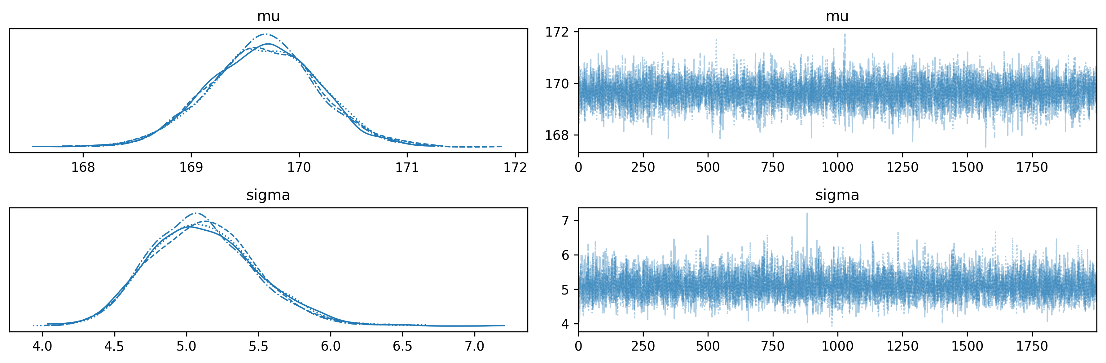

What to look for:

• Left panels: The distributions from all four chains should overlap almost perfectly. If they do not, the chains disagree.
• Right panels: The traces should look like “hairy caterpillars” —dense, well-mixed, with no long excursions or stuck periods. If you see a chain getting stuck at one value for many iterations, that is a problem.

2.6.2 Posterior Plot

A cleaner view of just the posterior distributions:

az.plot_posterior(
    idata,
    var_names=["mu", "sigma"],
    ref_val=[true_mu, true_sigma],
)
plt.tight_layout()
plt.show()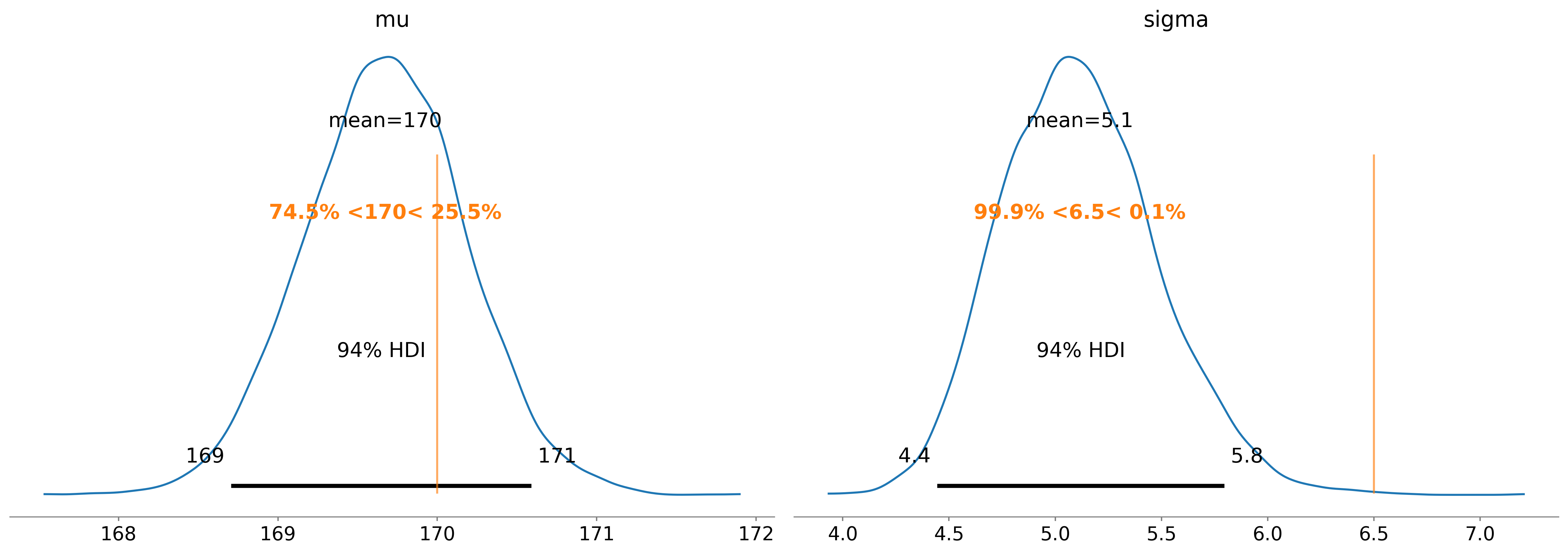

The ref_val argument adds vertical lines at the true values so you can see how well the model recovered them. In a real analysis you would not have true values, but during development with simulated data this check is essential.

2.6.3 Forest Plot

Forest plots are most useful when you have many parameters (for example, group-level effects in a hierarchical model). For our two-parameter model, they are overkill, but let us see the syntax:

az.plot_forest(idata, var_names=["mu", "sigma"])
plt.tight_layout()
plt.show()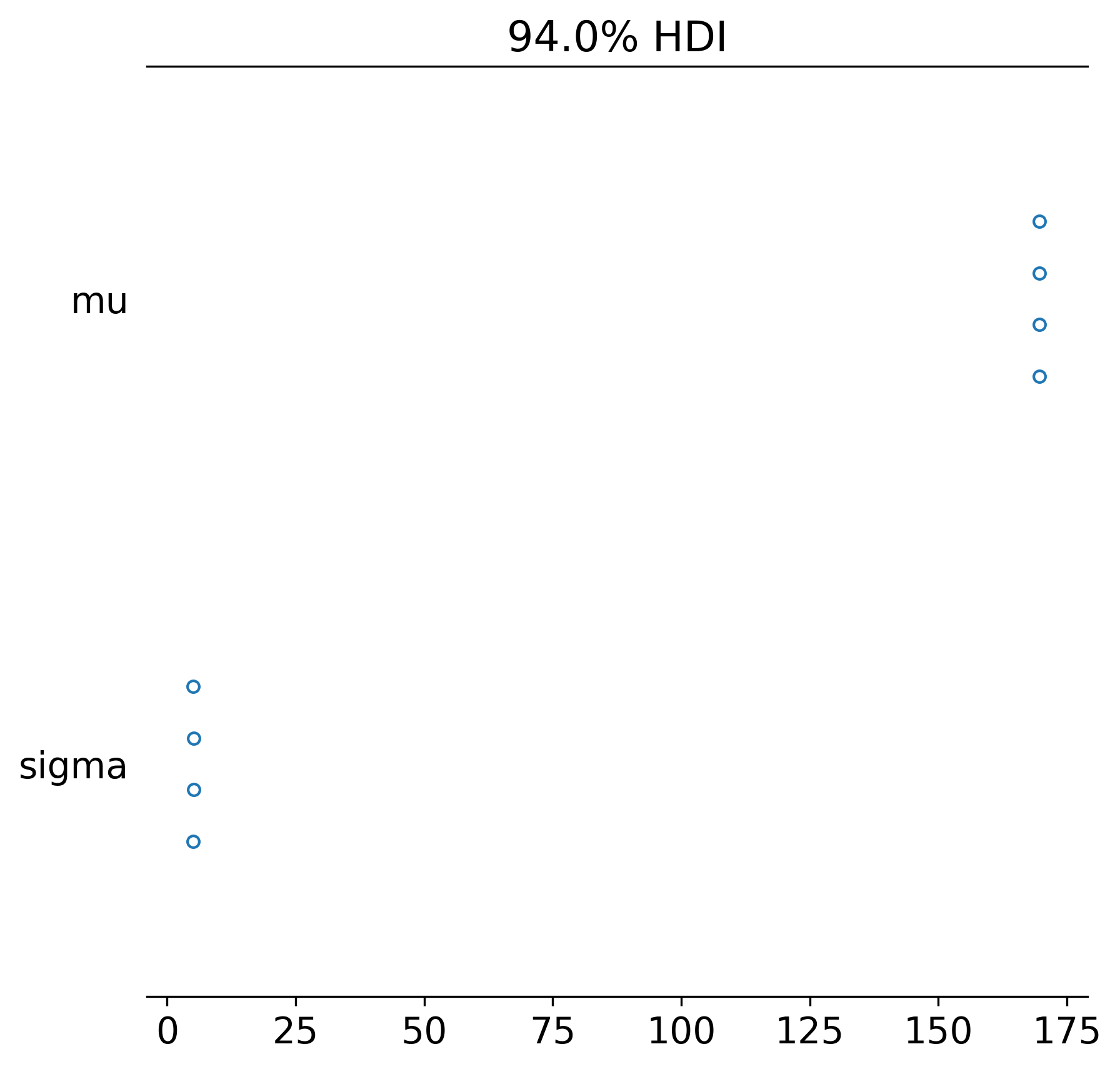

Each row shows the posterior interval for one parameter. The thick line is the inner credible interval, the thin line the outer. The dot is the posterior mean.

2.6.4 Which Plot When?

A quick reference for choosing the right visualisation:

Question	Plot
Did my sampler converge?	az.plot_trace()
What does the posterior look like?	az.plot_posterior()
How do parameters compare?	az.plot_forest()
Does my model fit the data?	az.plot_ppc()
Are there sampling problems?	az.plot_energy()
How correlated are parameters?	az.plot_pair()

Let us see one more useful plot—the pair plot, which shows correlations between parameters:

az.plot_pair(
    idata,
    var_names=["mu", "sigma"],
    kind="kde",
    marginals=True,
    figsize=(6, 6),
)
plt.tight_layout()
plt.show()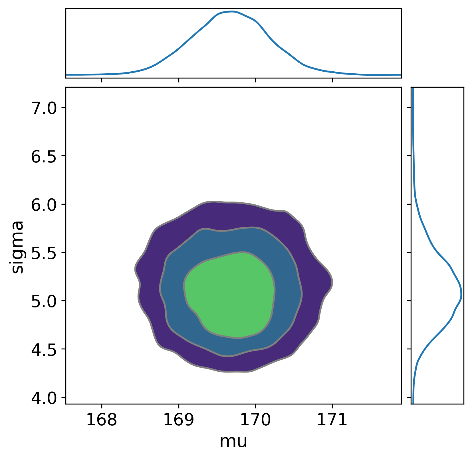

The pair plot shows the joint posterior of mu and sigma. If the contours are elongated (like a tilted ellipse), the parameters are correlated—knowing one tells you something about the other. For this simple model, the correlation is typically weak.

2.7 Prior Predictive Checks

Before you look at data, ask: “Does my model generate plausible data?” If your priors are badly chosen, the model can generate nonsensical predictions even before fitting. Prior predictive checks catch this.

The idea is simple. Take your model’s priors, ignore the observed data, and simulate datasets from those priors alone. If those simulated datasets look nothing like what you would expect to observe in reality, your priors need adjustment.

with height_model:
    prior_pred = pm.sample_prior_predictive(
        samples=500,
        random_seed=42,
    )

fig, axes = plt.subplots(nrows=1, ncols=2, figsize=(10, 4))

# Prior distributions of parameters
axes[0].hist(
    prior_pred.prior["mu"].values.flatten(),
    bins=30,
    alpha=0.7,
    color="steelblue",
)
axes[0].set_xlabel("mu (cm)")
axes[0].set_title("Prior on mu")

# Simulated data from the prior
prior_y = prior_pred.prior_predictive["y_obs"].values.flatten()
axes[1].hist(
    prior_y[np.isfinite(prior_y)],
    bins=50,
    alpha=0.7,
    color="coral",
    range=(100, 250),
)
axes[1].set_xlabel("Height (cm)")
axes[1].set_title("Prior predictive data")

plt.tight_layout()
plt.show()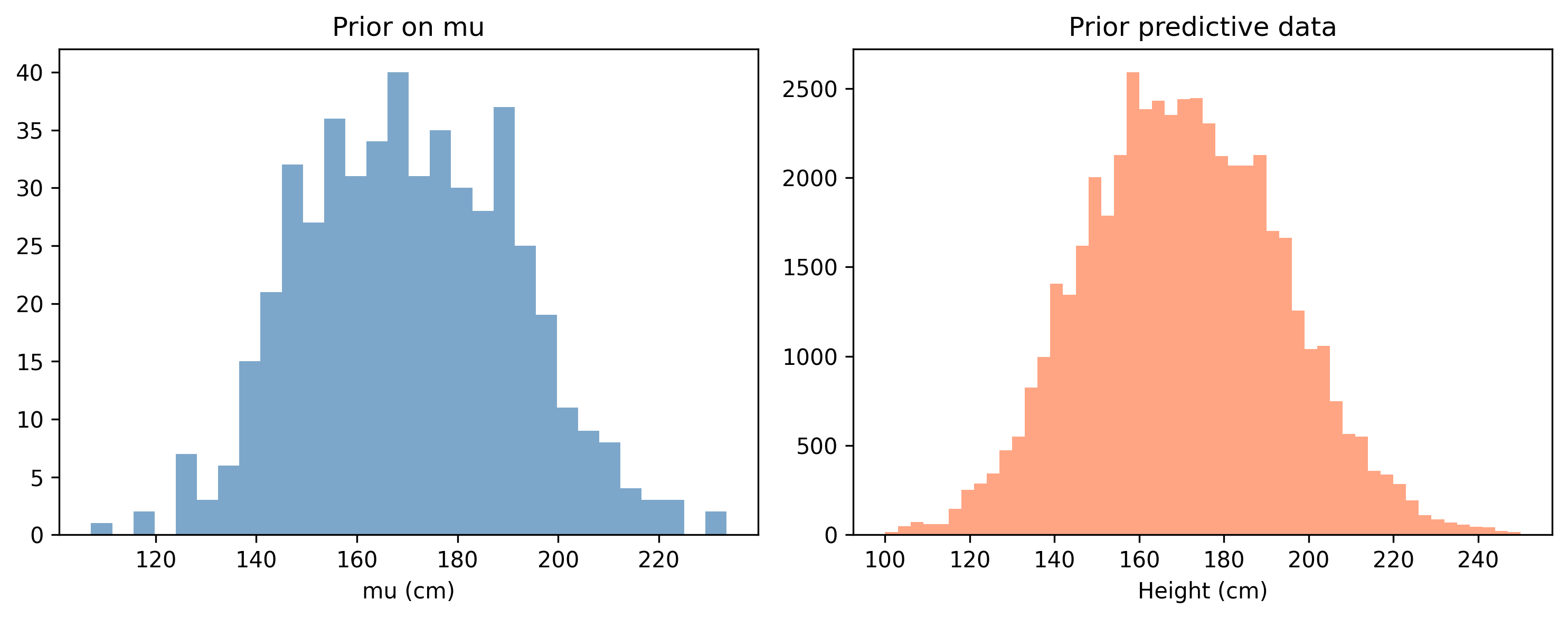

What to look for: The prior predictive data should cover the range of values you might plausibly observe. For heights, anything between 140 and 200 cm is reasonable. If your prior predictive generates heights of 500 cm or -100 cm with non-trivial probability, your priors are too vague.

Our priors are intentionally wide (sigma=20 on mu), so the prior predictive will span a broad range. That is fine—we want the data to do most of the work. What we do not want is for the priors to be so extreme that sampling becomes difficult.

2.7.1 A Practical Prior Predictive Workflow

Here is how experienced modellers use prior predictive checks in practice:

1. Define your model with initial priors. Start with something reasonable based on domain knowledge.
2. Run pm.sample_prior_predictive(). Generate, say, 500 simulated datasets.
3. Ask: “Would I be surprised to see any of these datasets in real life?” If yes, your priors are too vague. Tighten them.
4. Ask: “Could these priors exclude the real data?” If the prior predictive never generates data in the range you actually observe, your priors are too tight. Widen them.
5. Iterate until the prior predictive generates data that is plausible but varied. You want a range that covers reality without insisting on any particular outcome.

This is not about getting the priors “right” on the first try. It is about catching obviously wrong priors before you waste time sampling. A prior that generates heights of -50 cm is wrong. A prior that generates heights between 100 and 240 cm is fine—it is vague but not absurd.

2.7.2 Common Prior Predictive Failures

• All predictions are the same value: You accidentally used a very narrow prior (e.g., sigma=0.01 on your Normal prior). The prior is so confident it leaves no room for learning.
• Predictions span an absurd range (heights from -1000 to +1000): Your priors are far too vague. The model may technically converge, but it is not using your domain knowledge.
• The likelihood’s shape is wrong: You used a Normal likelihood for count data, so the prior predictive generates negative counts. Switch to Poisson or NegativeBinomial.

2.8 Posterior Predictive Checks

Posterior predictive checks are the single most important model validation tool. After fitting, you ask: “Can my fitted model generate data that looks like the real data?”

The logic: draw parameter values from the posterior, then simulate new data from the likelihood using those parameter values. If the simulated data matches the real data’s patterns (shape, spread, skewness), the model is adequate. If not, something is wrong.

with height_model:
    posterior_pred = pm.sample_posterior_predictive(
        idata,
        random_seed=42,
    )

/Users/kundeng/Dropbox/Projects/bayeslearner-learn-pymc/.venv/lib/python3.10/site-packages/rich/live.py:260: 
UserWarning: install "ipywidgets" for Jupyter support
  warnings.warn('install "ipywidgets" for Jupyter support')

az.plot_ppc(
    posterior_pred,
    observed_rug=True,
    figsize=(8, 4),
)
plt.xlabel("Height (cm)")
plt.title("Posterior Predictive Check")
plt.show()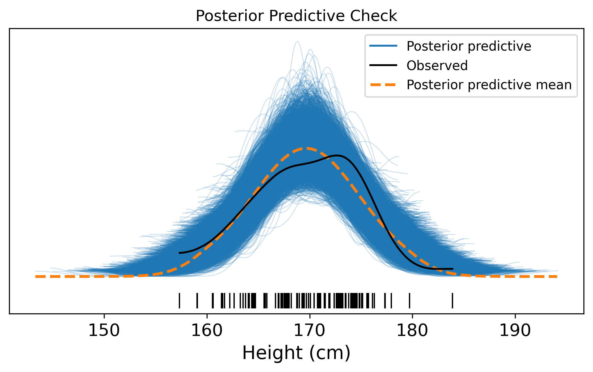

Reading the plot:

• The dark line is the observed data’s distribution.
• The light lines are simulated datasets from the posterior.
• If the simulated datasets envelope the observed data well, the model captures the data-generating process.
• If the observed data falls outside the simulated envelope—for example, if the real data is bimodal but the simulations are all unimodal—the model is missing something.

2.8.1 When Posterior Predictive Checks Fail

Common failures and what they mean:

• Simulated data is too narrow: Your model underestimates variability. Consider a heavier-tailed likelihood (Student-t instead of Normal).
• Simulated data is too wide: Your priors are too vague, or you have too little data. This is less common after fitting.
• Shape mismatch: The observed data has structure (bimodality, skewness) that your model cannot produce. You need a more flexible model.

2.8.2 Quantitative Posterior Predictive Checks

The visual az.plot_ppc() is a qualitative check. For a more rigorous assessment, you can compute test statistics on both the real data and the simulated data, then compare:

# Get posterior predictive samples
pp_samples = posterior_pred.posterior_predictive[
    "y_obs"
].values.reshape(-1, n_obs)

# Compute a test statistic on each simulated dataset
simulated_stds = pp_samples.std(axis=1)
observed_std = heights.std()

fig, ax = plt.subplots(figsize=(7, 4))
ax.hist(
    simulated_stds,
    bins=30,
    alpha=0.7,
    color="steelblue",
    edgecolor="white",
    label="Simulated",
)
ax.axvline(
    x=observed_std,
    color="red",
    linewidth=2,
    linestyle="--",
    label=f"Observed std = {observed_std:.2f}",
)
ax.set_xlabel("Standard deviation of dataset")
ax.set_ylabel("Frequency")
ax.set_title("Posterior Predictive Check: Std Dev")
ax.legend()
plt.tight_layout()
plt.show()

# Bayesian p-value: proportion of simulations
# with std > observed std
p_value = (simulated_stds >= observed_std).mean()
print(f"Bayesian p-value (std): {p_value:.3f}")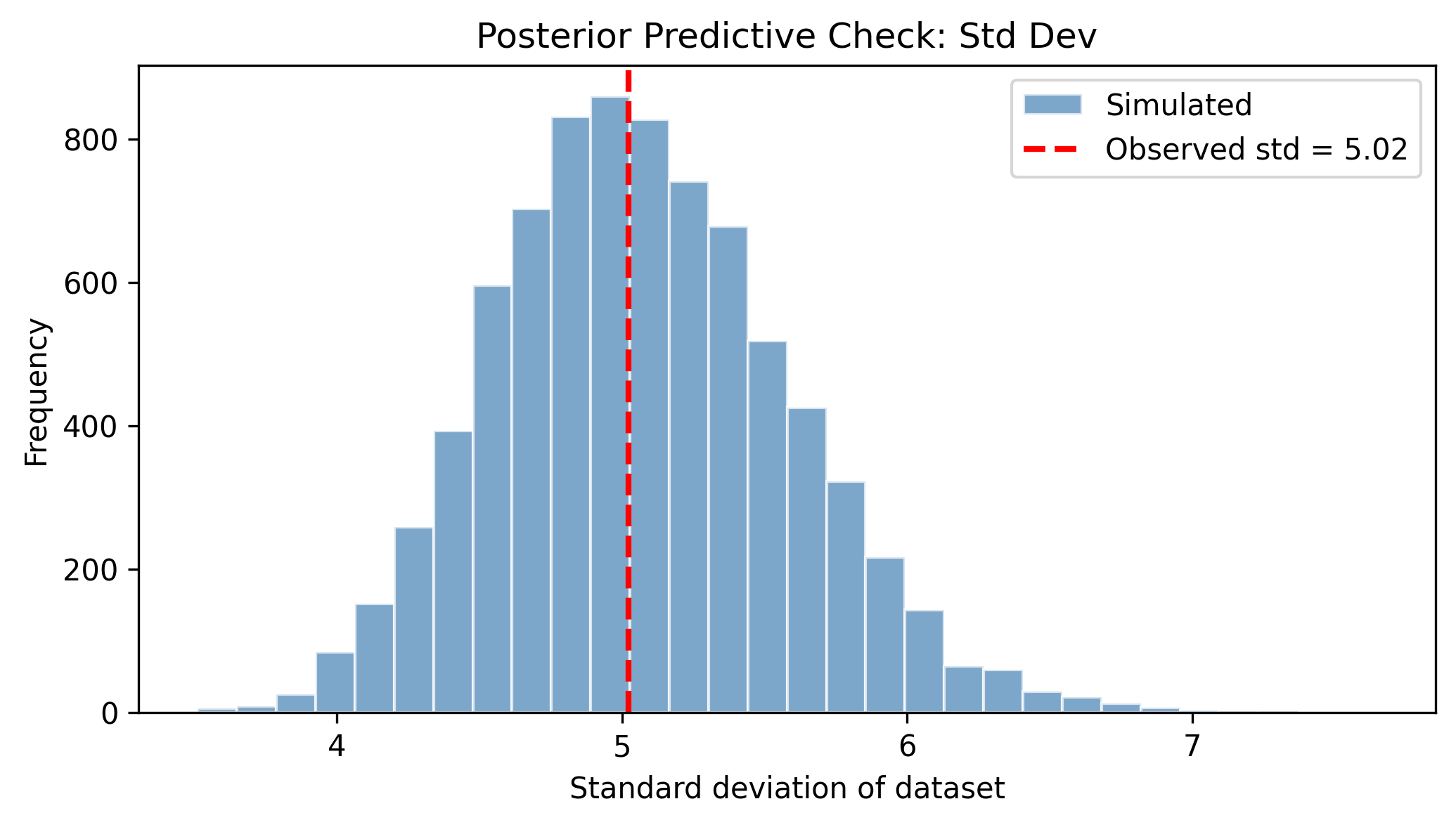

Bayesian p-value (std): 0.515

A Bayesian p-value near 0.5 is ideal—it means the observed test statistic sits in the middle of the predictive distribution. Values near 0 or 1 indicate the model systematically under- or over-predicts that aspect of the data.

2.8.3 The Prior-Posterior Comparison

A useful practice is to compare priors and posteriors directly. This shows how much the data moved your beliefs:

fig, axes = plt.subplots(nrows=1, ncols=2, figsize=(10, 4))

# mu: prior vs posterior
prior_mu = prior_pred.prior["mu"].values.flatten()
post_mu = idata.posterior["mu"].values.flatten()
axes[0].hist(
    prior_mu, bins=40, alpha=0.5, density=True,
    color="gray", label="Prior",
)
axes[0].hist(
    post_mu, bins=40, alpha=0.7, density=True,
    color="steelblue", label="Posterior",
)
axes[0].set_xlabel("mu")
axes[0].set_title("Prior vs Posterior: mu")
axes[0].legend()

# sigma: prior vs posterior
prior_sigma = prior_pred.prior["sigma"].values.flatten()
post_sigma = idata.posterior["sigma"].values.flatten()
axes[1].hist(
    prior_sigma, bins=40, alpha=0.5, density=True,
    color="gray", label="Prior",
)
axes[1].hist(
    post_sigma, bins=40, alpha=0.7, density=True,
    color="steelblue", label="Posterior",
)
axes[1].set_xlabel("sigma")
axes[1].set_title("Prior vs Posterior: sigma")
axes[1].legend()

plt.tight_layout()
plt.show()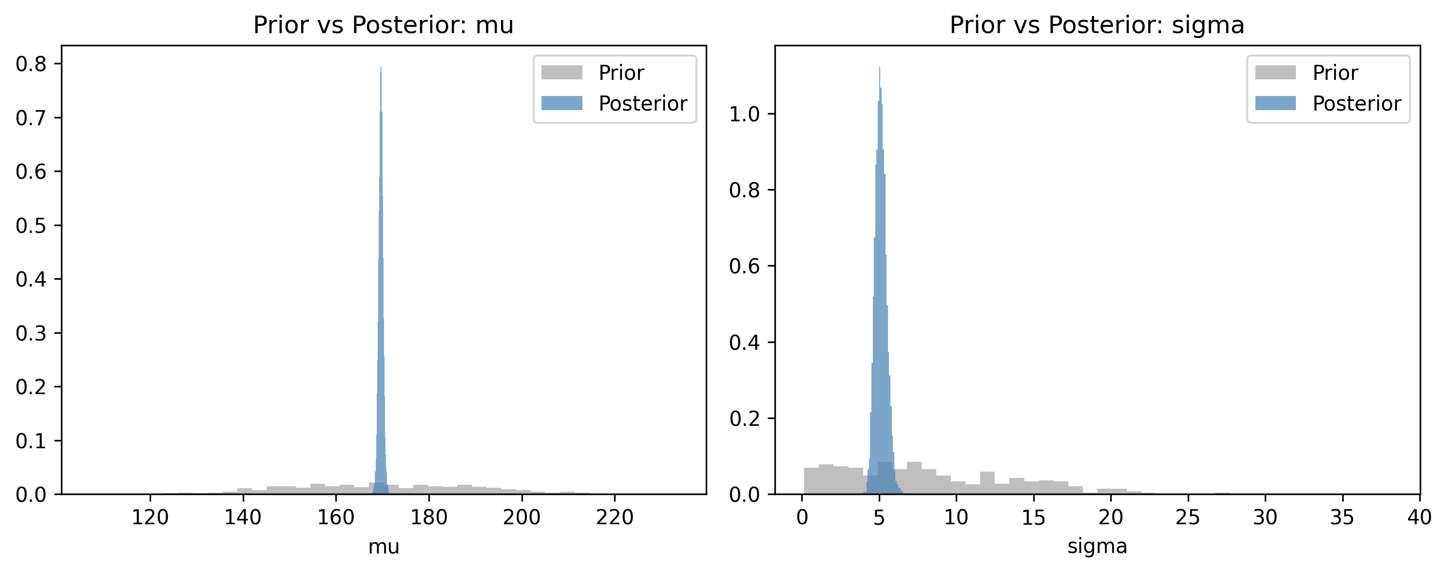

Notice how much narrower the posteriors are compared to the priors. With 100 data points, the data dominates the prior. The posterior concentrates tightly around the true values. This is learning: the data sharpened our beliefs from “somewhere between 130 and 210” to “almost certainly between 168 and 172.”

2.9 Deterministic Variables and Derived Quantities

Sometimes you want to track a computed quantity that depends on your parameters but is not itself a random variable. For example, the difference between two group means, or a predicted probability.

pm.Deterministic() tells PyMC: “Record this quantity in the trace so I can inspect it later.”

# Suppose we want to know: what fraction of the population
# is taller than 180 cm?

with pm.Model() as height_model_v2:
    mu = pm.Normal("mu", mu=170, sigma=20)
    sigma = pm.HalfNormal("sigma", sigma=10)

    # Derived quantity: probability of being > 180 cm
    # Using the normal CDF (complementary)
    from pytensor.tensor import erfc

    z_score = (180 - mu) / (sigma * np.sqrt(2))
    prob_above_180 = pm.Deterministic(
        "prob_above_180",
        0.5 * erfc(z_score),
    )

    y_obs = pm.Normal(
        "y_obs",
        mu=mu,
        sigma=sigma,
        observed=heights,
    )

    idata_v2 = pm.sample(
        draws=2000,
        tune=1000,
        chains=4,
        random_seed=42,
    )

/Users/kundeng/Dropbox/Projects/bayeslearner-learn-pymc/.venv/lib/python3.10/site-packages/rich/live.py:260: 
UserWarning: install "ipywidgets" for Jupyter support
  warnings.warn('install "ipywidgets" for Jupyter support')

az.plot_posterior(idata_v2, var_names=["prob_above_180"])
plt.title("Posterior: P(height > 180 cm)")
plt.show()

prob_summary = az.summary(
    idata_v2, var_names=["prob_above_180"]
)
print(prob_summary)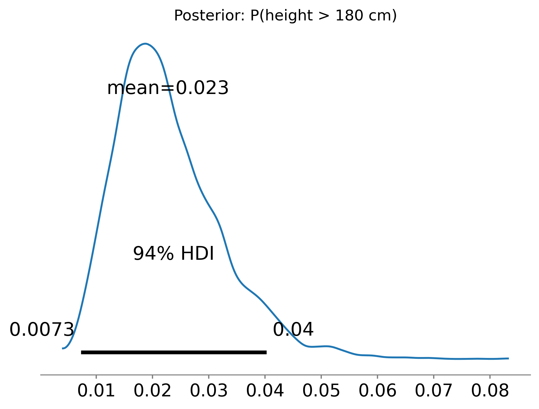

                 mean     sd  hdi_3%  hdi_97%  mcse_mean  mcse_sd  ess_bulk  \
prob_above_180  0.023  0.009   0.007     0.04        0.0      0.0    7566.0   

                ess_tail  r_hat  
prob_above_180    5483.0    1.0  

Without pm.Deterministic, you could compute this after the fact from the mu and sigma samples. But pm.Deterministic is cleaner: it stores the derived quantity directly in the trace, so it appears in summaries and plots automatically.

When to use pm.Deterministic:

• Any quantity you want to report or plot that is a function of model parameters.
• Differences between groups (pm.Deterministic("diff", mu_A - mu_B)).
• Predicted probabilities in logistic regression.
• Any intermediate computation that helps you interpret the model.

When not to use it:

• Simple transformations you only need once after fitting. Just compute them from the trace.
• Every single intermediate variable—this bloats the trace. Only track quantities you actually want to inspect.

2.10 Putting It All Together: The Full Workflow

Let us summarise the complete PyMC workflow in one coherent block. This is the pattern you will follow for every model in this book:

# ----- 1. Data -----
data = rng.normal(loc=5.0, scale=2.0, size=200)

# ----- 2. Model -----
with pm.Model() as workflow_model:
    # Priors
    mu = pm.Normal("mu", mu=0, sigma=10)
    sigma = pm.HalfNormal("sigma", sigma=5)

    # Likelihood
    obs = pm.Normal("obs", mu=mu, sigma=sigma, observed=data)

    # ----- 3. Prior predictive check -----
    prior_checks = pm.sample_prior_predictive(
        samples=500, random_seed=42
    )

    # ----- 4. Sample the posterior -----
    trace = pm.sample(
        draws=2000,
        tune=1000,
        chains=4,
        random_seed=42,
    )

    # ----- 5. Posterior predictive check -----
    ppc = pm.sample_posterior_predictive(
        trace, random_seed=42
    )

/Users/kundeng/Dropbox/Projects/bayeslearner-learn-pymc/.venv/lib/python3.10/site-packages/rich/live.py:260: 
UserWarning: install "ipywidgets" for Jupyter support
  warnings.warn('install "ipywidgets" for Jupyter support')

/Users/kundeng/Dropbox/Projects/bayeslearner-learn-pymc/.venv/lib/python3.10/site-packages/rich/live.py:260: 
UserWarning: install "ipywidgets" for Jupyter support
  warnings.warn('install "ipywidgets" for Jupyter support')

# ----- 6. Diagnostics -----
print(az.summary(trace, var_names=["mu", "sigma"]))

fig, axes = plt.subplots(nrows=2, ncols=2, figsize=(10, 6))

az.plot_trace(trace, var_names=["mu", "sigma"], axes=axes)
plt.tight_layout()
plt.show()

        mean     sd  hdi_3%  hdi_97%  mcse_mean  mcse_sd  ess_bulk  ess_tail  \
mu     4.925  0.142   4.659    5.190      0.002    0.002    7822.0    5842.0   
sigma  2.012  0.101   1.822    2.201      0.001    0.001    8348.0    6182.0   

       r_hat  
mu       1.0  
sigma    1.0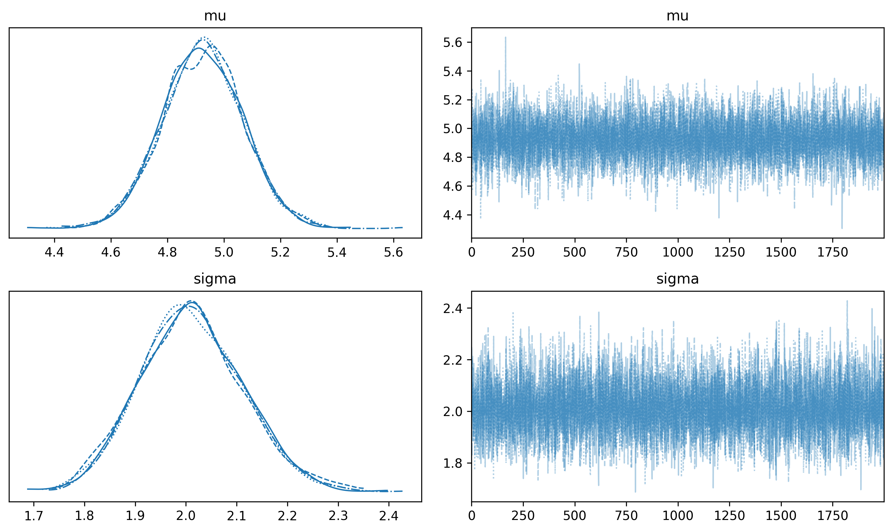  

# ----- 7. Posterior predictive plot -----
az.plot_ppc(ppc, figsize=(8, 4))
plt.title("Posterior Predictive Check")
plt.show()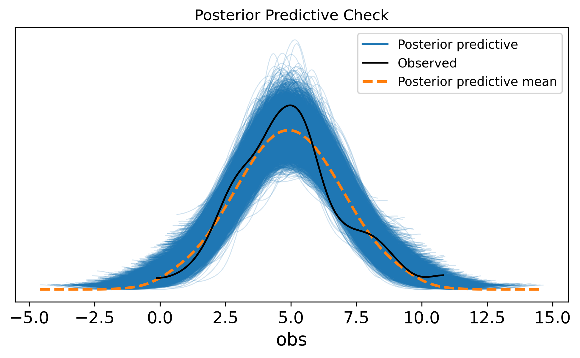

This seven-step sequence—data, model, prior check, sample, posterior check, diagnostics, interpretation—is the backbone of every Bayesian analysis. Some steps are quick (a glance at the trace plot). Others require thought (choosing priors, interpreting posterior predictive failures). But the sequence is always the same.

2.11 Exercises

Exercise 1. You flip a coin 50 times and observe 32 heads. Build a PyMC model that estimates the probability of heads. Use a pm.Beta prior and a pm.Binomial likelihood. Report the posterior mean and 94% HDI for the probability parameter.

Solution

n_flips = 50
n_heads = 32

with pm.Model() as coin_model:
    # Beta(2, 2) is a weakly informative prior:
    # slightly favours values near 0.5
    p = pm.Beta("p", alpha=2, beta=2)

    # Likelihood: observed 32 heads in 50 flips
    y = pm.Binomial(
        "y", n=n_flips, p=p, observed=n_heads
    )

    coin_trace = pm.sample(
        draws=2000,
        tune=1000,
        chains=4,
        random_seed=42,
    )

print(az.summary(coin_trace, var_names=["p"]))
az.plot_posterior(coin_trace, var_names=["p"])
plt.show()

/Users/kundeng/Dropbox/Projects/bayeslearner-learn-pymc/.venv/lib/python3.10/site-packages/rich/live.py:260: 
UserWarning: install "ipywidgets" for Jupyter support
  warnings.warn('install "ipywidgets" for Jupyter support')

   mean     sd  hdi_3%  hdi_97%  mcse_mean  mcse_sd  ess_bulk  ess_tail  r_hat
p  0.63  0.065   0.509    0.751      0.001    0.001    3464.0    5693.0    1.0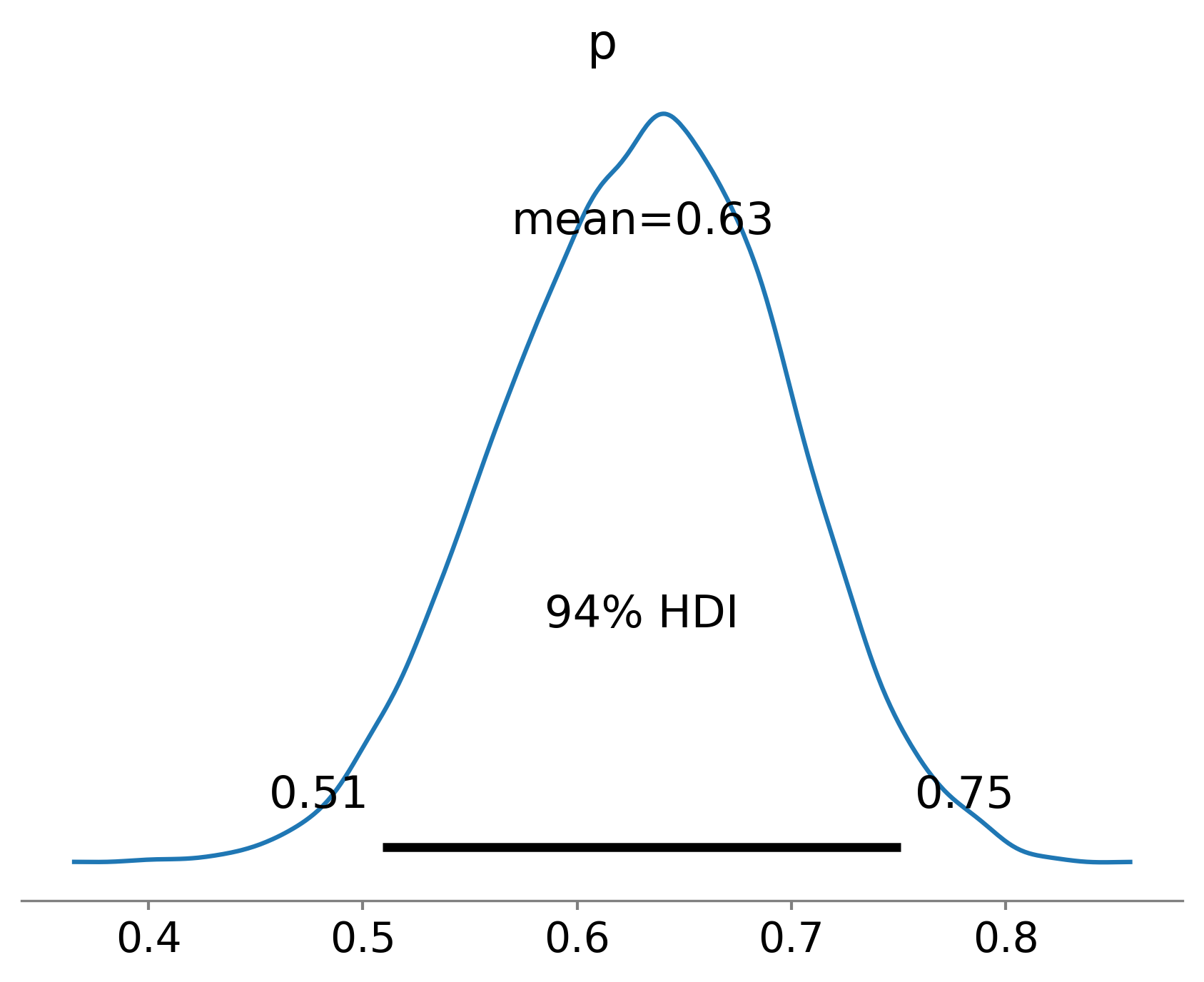

Exercise 2. Modify the height model from this chapter to use a Student-t likelihood instead of Normal. Use pm.StudentT with nu=4 degrees of freedom. Compare the posterior estimates of mu and sigma to the Normal-likelihood version. Which model has wider credible intervals? Why?

Solution

with pm.Model() as robust_model:
    mu = pm.Normal("mu", mu=170, sigma=20)
    sigma = pm.HalfNormal("sigma", sigma=10)

    # Student-t likelihood (heavier tails)
    y_obs = pm.StudentT(
        "y_obs",
        nu=4,
        mu=mu,
        sigma=sigma,
        observed=heights,
    )

    robust_trace = pm.sample(
        draws=2000,
        tune=1000,
        chains=4,
        random_seed=42,
    )

print("--- Student-t model ---")
print(az.summary(robust_trace, var_names=["mu", "sigma"]))
print("\n--- Normal model (from earlier) ---")
print(az.summary(idata, var_names=["mu", "sigma"]))

/Users/kundeng/Dropbox/Projects/bayeslearner-learn-pymc/.venv/lib/python3.10/site-packages/rich/live.py:260: 
UserWarning: install "ipywidgets" for Jupyter support
  warnings.warn('install "ipywidgets" for Jupyter support')

--- Student-t model ---
          mean     sd   hdi_3%  hdi_97%  mcse_mean  mcse_sd  ess_bulk  \
mu     169.866  0.523  168.885  170.834      0.006    0.006    7993.0   
sigma    4.370  0.390    3.614    5.073      0.005    0.004    7388.0   

       ess_tail  r_hat  
mu       5733.0    1.0  
sigma    5859.0    1.0  

--- Normal model (from earlier) ---
          mean     sd   hdi_3%  hdi_97%  mcse_mean  mcse_sd  ess_bulk  \
mu     169.673  0.506  168.707  170.591      0.006    0.006    7977.0   
sigma    5.115  0.367    4.444    5.796      0.004    0.004    7429.0   

       ess_tail  r_hat  
mu       5519.0    1.0  
sigma    5789.0    1.0  

The Student-t model typically produces slightly wider credible intervals because the heavier-tailed likelihood allows for more variation in the data. Each observation carries less “certainty” than it would under a Normal likelihood.

Exercise 3. Run a prior predictive check on the coin model from Exercise 1. Plot a histogram of simulated “number of heads” from the prior. Does the prior generate plausible data?

Solution

with coin_model:
    coin_prior = pm.sample_prior_predictive(
        samples=1000, random_seed=42
    )

prior_heads = (
    coin_prior.prior_predictive["y"].values.flatten()
)

fig, ax = plt.subplots(figsize=(7, 4))
ax.hist(
    prior_heads,
    bins=range(0, 52),
    alpha=0.7,
    color="steelblue",
    edgecolor="white",
)
ax.axvline(
    x=n_heads, color="red", linestyle="--",
    label=f"Observed ({n_heads} heads)",
)
ax.set_xlabel("Number of heads (out of 50)")
ax.set_ylabel("Frequency")
ax.set_title("Prior Predictive: Coin Model")
ax.legend()
plt.tight_layout()
plt.show()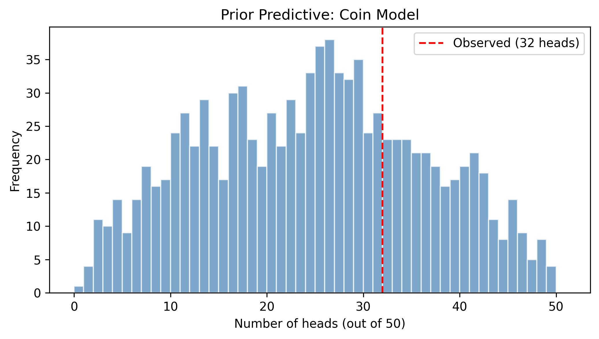

With a Beta(2, 2) prior, the model generates head counts spread across the full range 0–50, with a mild concentration near 25. This is reasonable: before seeing data, we are fairly uncertain but lean toward a fair coin. The observed value of 32 sits comfortably within the prior predictive range, confirming the prior is not excluding plausible outcomes.

Exercise 4. You measure the waiting time (in minutes) between buses at a stop. You record 20 observations: [4.2, 7.1, 3.8, 5.5, 6.3, 4.9, 8.2, 3.1, 5.8, 7.4, 4.6, 6.1, 5.3, 9.0, 4.4, 6.7, 3.5, 5.9, 7.8, 4.1]. Build a model assuming wait times follow an Exponential distribution. Use a pm.Gamma prior on the rate parameter. Sample the posterior, plot the trace, and run a posterior predictive check.

Solution

wait_times = np.array([
    4.2, 7.1, 3.8, 5.5, 6.3, 4.9, 8.2, 3.1,
    5.8, 7.4, 4.6, 6.1, 5.3, 9.0, 4.4, 6.7,
    3.5, 5.9, 7.8, 4.1,
])

with pm.Model() as bus_model:
    # Gamma(2, 1) prior on rate: mean=2, moderate uncertainty
    # rate = 1/mean_wait_time
    rate = pm.Gamma("rate", alpha=2, beta=10)

    # Exponential likelihood
    obs = pm.Exponential(
        "obs", lam=rate, observed=wait_times
    )

    bus_trace = pm.sample(
        draws=2000,
        tune=1000,
        chains=4,
        random_seed=42,
    )

    bus_ppc = pm.sample_posterior_predictive(
        bus_trace, random_seed=42
    )

# Diagnostics
print(az.summary(bus_trace, var_names=["rate"]))
az.plot_trace(bus_trace, var_names=["rate"])
plt.tight_layout()
plt.show()

# Posterior predictive check
az.plot_ppc(bus_ppc, figsize=(8, 4))
plt.title("PPC: Bus Wait Times")
plt.show()

/Users/kundeng/Dropbox/Projects/bayeslearner-learn-pymc/.venv/lib/python3.10/site-packages/rich/live.py:260: 
UserWarning: install "ipywidgets" for Jupyter support
  warnings.warn('install "ipywidgets" for Jupyter support')

/Users/kundeng/Dropbox/Projects/bayeslearner-learn-pymc/.venv/lib/python3.10/site-packages/rich/live.py:260: 
UserWarning: install "ipywidgets" for Jupyter support
  warnings.warn('install "ipywidgets" for Jupyter support')

       mean     sd  hdi_3%  hdi_97%  mcse_mean  mcse_sd  ess_bulk  ess_tail  \
rate  0.178  0.037   0.107    0.244      0.001      0.0    3136.0    4761.0   

      r_hat  
rate    1.0  

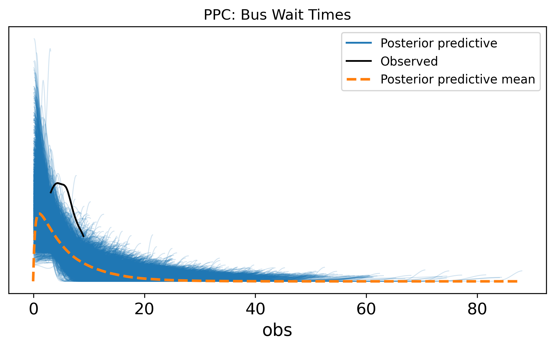
You may notice the posterior predictive check shows some mismatch—the Exponential distribution always peaks at zero, but the observed data peaks around 4–6 minutes. This suggests a Gamma or LogNormal likelihood might be more appropriate. Posterior predictive checks revealing model inadequacy is exactly how they are supposed to work.

Prediction without refitting: the mutable data pattern

A practical pattern Fonnesbeck highlights is mutable data. After fitting a model, you often want predictions on new inputs without re-running the sampler. PyMC’s pm.Data containers let you swap observed data after fitting:

with pm.Model() as model:
    x = pm.Data("x", x_train)
    # ... define priors and likelihood using x ...
    trace = pm.sample()

    # Swap in new data, no re-sampling needed
    pm.set_data({"x": x_new})
    ppc = pm.sample_posterior_predictive(trace)

This is critical for practical workflows — you fit once, then generate posterior predictive samples for as many new inputs as you like.

Turning the Bayesian crank

Fonnesbeck captures a key Bayesian insight: “You can always turn the Bayesian crank — take your posterior as the prior for new data.” This is sequential updating in action. When new data arrives, you do not start over; your posterior from the first batch of data becomes your prior for the second batch. The math guarantees that updating sequentially gives the same result as updating all at once (we proved this in Chapter 1, Exercise 1). In practice, this means Bayesian models learn continuously.

2.12 Chapter Summary

You now know the core PyMC workflow:

1. Define a model inside with pm.Model().
2. Specify priors for unknown parameters using PyMC distributions.
3. Connect data using observed= in the likelihood.
4. Check priors with pm.sample_prior_predictive().
5. Sample the posterior with pm.sample().
6. Diagnose with az.summary(), az.plot_trace(), and R-hat/ESS.
7. Validate with pm.sample_posterior_predictive() and az.plot_ppc().
8. Track derived quantities with pm.Deterministic().

In the next chapter, we put this workflow to use on a real modelling problem: linear regression, the Bayesian way.